Chapter 9 Analyse data

We’ll just very briefly go into doing analyses in R. We’ll combine it with other stuff we have learned today.

9.1 t-tests

t-tests are also easily done with the t.test()-function. Let’s examine whether cars in 2008 are more efficient than cars in 1997. Let’s first see some descriptives:

df %>% select(year, cty) %>% group_by(year) %>% skim

Table 9.1: Data summary
Name	Piped data
Number of rows	234
Number of columns	2
_______________________
Column type frequency:
numeric	1
________________________
Group variables	year

Variable type: numeric

skim_variable	year	n_missing	complete_rate	mean	sd	p0	p25	p50	p75	p100	hist
cty	1999	0	1	17.02	4.46	11	14	17	19	35	▇▇▃▁▁
cty	2008	0	1	16.70	4.06	9	13	17	20	28	▃▇▇▃▁

Similar means and medians. If anything, cars are less fuel efficient in 2008

`?t.test’ provides you with help on how to use it. Let’s assume equal variances in both groups, giving us a nice round number of degrees of freedom.

t.test(cty ~ year, data = df, var.equal = TRUE)

## 
##  Two Sample t-test
## 
## data:  cty by year
## t = 0.5675, df = 232, p-value = 0.5709
## alternative hypothesis: true difference in means between group 1999 and group 2008 is not equal to 0
## 95 percent confidence interval:
##  -0.781680  1.414159
## sample estimates:
## mean in group 1999 mean in group 2008 
##           17.01709           16.70085

9.2 ANOVA

Let’s say we are interested in the association between the type of car (front-, rear-, or fourwheel drive measured by drv) and its fuel efficiency in cities (measured by cty). Let’s get a bit of background info on the variables first.

df %>% select(cty, drv) %>% skim

Table 9.2: Data summary
Name	Piped data
Number of rows	234
Number of columns	2
_______________________
Column type frequency:
character	1
numeric	1
________________________
Group variables	None

Variable type: character

skim_variable	n_missing	complete_rate	min	max	empty	n_unique	whitespace
drv	0	1	1	1	0	3	0

Variable type: numeric

skim_variable	n_missing	complete_rate	mean	sd	p0	p25	p50	p75	p100	hist
cty	0	1	16.86	4.26	9	14	17	19	35	▆▇▃▁▁

We can see that our drv variable has three groups. Let’s see a frequency table of this variable:

table(df$drv)

## 
##   4   f   r 
## 103 106  25

Relatively few rearwheeldrives. Let’s look at the summary statistics of cty for each drv group:

df %>% select(cty, drv) %>% group_by(drv) %>% skim

Table 9.3: Data summary
Name	Piped data
Number of rows	234
Number of columns	2
_______________________
Column type frequency:
numeric	1
________________________
Group variables	drv

Variable type: numeric

skim_variable	drv	complete_rate	mean	sd	p0	p25	p50	p75	p100	hist
cty	4	1	14.33	2.87	9	13	14	16	21	▅▆▇▂▃
cty	f	1	19.97	3.63	11	18	19	21	35	▁▇▅▁▁
cty	r	1	14.08	2.22	11	12	15	15	18	▆▁▇▂▂

The mean efficieny is much higher for the “f” compared to the other categories. Let’s visualise this ourselves:

ggplot(df, aes(x=drv, y=cty)) + 
  geom_violin() + 
  geom_jitter(width = 0.1, height = 0)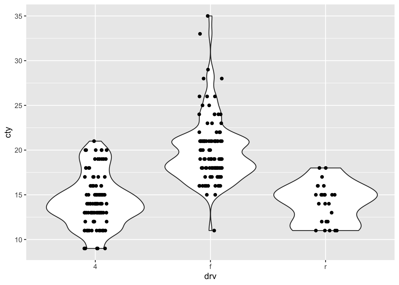

it’s also very clear from the graph that the distribution of “f” is shifted upwards compared to the other categories. There is also more variation in the “f” category.

Let’s do an ANOVA:

mod_anova <- aov(cty ~ drv, data=df)
summary(mod_anova)

##              Df Sum Sq Mean Sq F value Pr(>F)    
## drv           2   1879   939.4   92.68 <2e-16 ***
## Residuals   231   2342    10.1                   
## ---
## Signif. codes:  0 '***' 0.001 '**' 0.01 '*' 0.05 '.' 0.1 ' ' 1

Post-hoc comparisons:

TukeyHSD(mod_anova)

##   Tukey multiple comparisons of means
##     95% family-wise confidence level
## 
## Fit: aov(formula = cty ~ drv, data = df)
## 
## $drv
##           diff       lwr       upr     p adj
## f-4  5.6416010  4.602497  6.680705 0.0000000
## r-4 -0.2500971 -1.924554  1.424359 0.9338857
## r-f -5.8916981 -7.561520 -4.221876 0.0000000

9.3 Linear regression

We also could have done the above analysis through a linear regression:

mod1 <- lm(cty ~ drv, data = mpg)
summary(mod1)

## 
## Call:
## lm(formula = cty ~ drv, data = mpg)
## 
## Residuals:
##     Min      1Q  Median      3Q     Max 
## -8.9717 -1.9717 -0.3301  1.0283 15.0283 
## 
## Coefficients:
##             Estimate Std. Error t value Pr(>|t|)    
## (Intercept)  14.3301     0.3137  45.680   <2e-16 ***
## drvf          5.6416     0.4405  12.807   <2e-16 ***
## drvr         -0.2501     0.7098  -0.352    0.725    
## ---
## Signif. codes:  0 '***' 0.001 '**' 0.01 '*' 0.05 '.' 0.1 ' ' 1
## 
## Residual standard error: 3.184 on 231 degrees of freedom
## Multiple R-squared:  0.4452, Adjusted R-squared:  0.4404 
## F-statistic: 92.68 on 2 and 231 DF,  p-value: < 2.2e-16

Our regression model object (mod1) contains much more useful information. Let’s have a look:

str(mod1)

## List of 13
##  $ coefficients : Named num [1:3] 14.33 5.64 -0.25
##   ..- attr(*, "names")= chr [1:3] "(Intercept)" "drvf" "drvr"
##  $ residuals    : Named num [1:234] -1.9717 1.0283 0.0283 1.0283 -3.9717 ...
##   ..- attr(*, "names")= chr [1:234] "1" "2" "3" "4" ...
##  $ effects      : Named num [1:234] -257.89 -43.33 -1.12 1.08 -3.92 ...
##   ..- attr(*, "names")= chr [1:234] "(Intercept)" "drvf" "drvr" "" ...
##  $ rank         : int 3
##  $ fitted.values: Named num [1:234] 20 20 20 20 20 ...
##   ..- attr(*, "names")= chr [1:234] "1" "2" "3" "4" ...
##  $ assign       : int [1:3] 0 1 1
##  $ qr           :List of 5
##   ..$ qr   : num [1:234, 1:3] -15.2971 0.0654 0.0654 0.0654 0.0654 ...
##   .. ..- attr(*, "dimnames")=List of 2
##   .. .. ..$ : chr [1:234] "1" "2" "3" "4" ...
##   .. .. ..$ : chr [1:3] "(Intercept)" "drvf" "drvr"
##   .. ..- attr(*, "assign")= int [1:3] 0 1 1
##   .. ..- attr(*, "contrasts")=List of 1
##   .. .. ..$ drv: chr "contr.treatment"
##   ..$ qraux: num [1:3] 1.07 1.07 1
##   ..$ pivot: int [1:3] 1 2 3
##   ..$ tol  : num 1e-07
##   ..$ rank : int 3
##   ..- attr(*, "class")= chr "qr"
##  $ df.residual  : int 231
##  $ contrasts    :List of 1
##   ..$ drv: chr "contr.treatment"
##  $ xlevels      :List of 1
##   ..$ drv: chr [1:3] "4" "f" "r"
##  $ call         : language lm(formula = cty ~ drv, data = mpg)
##  $ terms        :Classes 'terms', 'formula'  language cty ~ drv
##   .. ..- attr(*, "variables")= language list(cty, drv)
##   .. ..- attr(*, "factors")= int [1:2, 1] 0 1
##   .. .. ..- attr(*, "dimnames")=List of 2
##   .. .. .. ..$ : chr [1:2] "cty" "drv"
##   .. .. .. ..$ : chr "drv"
##   .. ..- attr(*, "term.labels")= chr "drv"
##   .. ..- attr(*, "order")= int 1
##   .. ..- attr(*, "intercept")= int 1
##   .. ..- attr(*, "response")= int 1
##   .. ..- attr(*, ".Environment")=<environment: R_GlobalEnv> 
##   .. ..- attr(*, "predvars")= language list(cty, drv)
##   .. ..- attr(*, "dataClasses")= Named chr [1:2] "numeric" "character"
##   .. .. ..- attr(*, "names")= chr [1:2] "cty" "drv"
##  $ model        :'data.frame':   234 obs. of  2 variables:
##   ..$ cty: int [1:234] 18 21 20 21 16 18 18 18 16 20 ...
##   ..$ drv: chr [1:234] "f" "f" "f" "f" ...
##   ..- attr(*, "terms")=Classes 'terms', 'formula'  language cty ~ drv
##   .. .. ..- attr(*, "variables")= language list(cty, drv)
##   .. .. ..- attr(*, "factors")= int [1:2, 1] 0 1
##   .. .. .. ..- attr(*, "dimnames")=List of 2
##   .. .. .. .. ..$ : chr [1:2] "cty" "drv"
##   .. .. .. .. ..$ : chr "drv"
##   .. .. ..- attr(*, "term.labels")= chr "drv"
##   .. .. ..- attr(*, "order")= int 1
##   .. .. ..- attr(*, "intercept")= int 1
##   .. .. ..- attr(*, "response")= int 1
##   .. .. ..- attr(*, ".Environment")=<environment: R_GlobalEnv> 
##   .. .. ..- attr(*, "predvars")= language list(cty, drv)
##   .. .. ..- attr(*, "dataClasses")= Named chr [1:2] "numeric" "character"
##   .. .. .. ..- attr(*, "names")= chr [1:2] "cty" "drv"
##  - attr(*, "class")= chr "lm"

Woah there is a lot information in the mod1 object. But it’s not stored very conveniently. We can get to the residuals by using mod1$residuals. Let’s plot them:

# We need to store the residuals in dataframe first
resid_df <- data.frame(residuals = mod1$residuals)
ggplot(resid_df, aes(x = residuals)) + geom_histogram(binwidth = 1)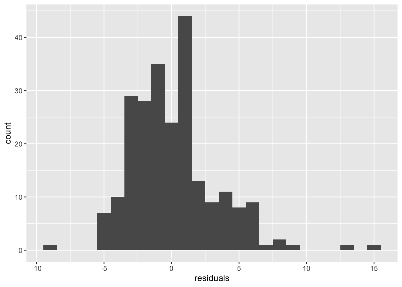

Not too bad. Combined with the large sample size, we probably don’t need to worry about the model assumptions too much.

9.4 Chi-square

For testing whether two categorial variables are (in)dependent, we can use the chi-square-test. Let’s examine the association between year (1997, 2008) and type of drive (front, rear, or fourwheeldrive)

table(df$year, df$drv)

##       
##         4  f  r
##   1999 49 57 11
##   2008 54 49 14

The test:

chisq.test(df$drv, df$year, correct = FALSE)

## 
##  Pearson's Chi-squared test
## 
## data:  df$drv and df$year
## X-squared = 1.2065, df = 2, p-value = 0.547

9.5 More advanced analyses

There is little time today to cover the diversity of statistical methods that are out there, so we’ll just give a quick overview of some topics that might be of interest, and relevant R-packages. State-of-the-art analysis functionality is a major strength of R

9.5.1 Multilevel models

library(lme4)
library(nlme)

9.5.2 Cronbach’s alpha

library(alpha)
# With the function
alpha(your_data)

9.5.3 Principal component analysis

library(psych)
# With the function
principal(your_data)

9.5.4 Factor analysis

library(psych)
# With the function
fa(your_data)

9.5.5 Structural equation modeling

library(lavaan)

9.5.6 Item response theory

library(irtoys)
library(ltm)

9.5.7 Bayesian analysis

The choice is immense with respect to bayesian analysis: https://cran.r-project.org/web/views/Bayesian.html. Still some prominent examples:

library(Rstan)
library(rjags)

9.6 Further reading

The analysis-chapter in the R for Data Science book may be useful: http://r4ds.had.co.nz/model-intro.html. Also, for more information on the broom-package, see: https://cran.r-project.org/web/packages/broom/vignettes/broom.html

Chapter 9 Analyse data

9.1 t-tests

9.2 ANOVA

9.3 Linear regression

9.4 Chi-square

9.5 More advanced analyses

9.5.1 Multilevel models

9.5.2 Cronbach’s alpha

9.5.3 Principal component analysis

9.5.4 Factor analysis

9.5.5 Structural equation modeling

9.5.6 Item response theory

9.5.7 Bayesian analysis

9.5.8 Social network analysis

9.6 Further reading