Chapter 7 Transform data

Now onto the really exciting stuff; transforming/manipulating/wrangling our data! Often we need to create new variables or create subsets of our dataframe (selecting particular variables or cases) before we can visualise and analyse. We’ll do this by using the functions provided in the dplyr package, that are much more intuitive and consistent to use than the base R-functions. To be able to make use of the dplyr-package, we have to install it and load it. Instead, we’ll install and load the tidyverse-package (Wickham (2017)), this is a collection of packages (including dplyr) that are extremely useful.

library(tidyverse)

We’ll focus on four functions:

1. select() which allows you to select variables (or columns)

2. filter() which allows you to select cases (or rows)

3. mutate() which allows you to create new variables

4. summarise() which allows you to summarise variables

We shall make use of a built-in dataset called mpg of the ggplot2-package (which is automatically loaded in the tidyverse). This dataset describes “Fuel economy data from 1999 and 2008 for 38 popular models of car” (http://ggplot2.tidyverse.org/reference/mpg.html)

df <- mpg

Let’s take a look at our dataset df that is now in our Global Environment, by clicking on it. Subsequently, run this code:

str(df)

## tibble [234 × 11] (S3: tbl_df/tbl/data.frame)
##  $ manufacturer: chr [1:234] "audi" "audi" "audi" "audi" ...
##  $ model       : chr [1:234] "a4" "a4" "a4" "a4" ...
##  $ displ       : num [1:234] 1.8 1.8 2 2 2.8 2.8 3.1 1.8 1.8 2 ...
##  $ year        : int [1:234] 1999 1999 2008 2008 1999 1999 2008 1999 1999 2008 ...
##  $ cyl         : int [1:234] 4 4 4 4 6 6 6 4 4 4 ...
##  $ trans       : chr [1:234] "auto(l5)" "manual(m5)" "manual(m6)" "auto(av)" ...
##  $ drv         : chr [1:234] "f" "f" "f" "f" ...
##  $ cty         : int [1:234] 18 21 20 21 16 18 18 18 16 20 ...
##  $ hwy         : int [1:234] 29 29 31 30 26 26 27 26 25 28 ...
##  $ fl          : chr [1:234] "p" "p" "p" "p" ...
##  $ class       : chr [1:234] "compact" "compact" "compact" "compact" ...

There are a bunch of numerical values (num and int) and many character values (chr).

7.1 The pipe: %>%

We’ll now learn a weird bit of coding that makes it much more easy to ‘read’ and understand your code (also for future you!). We’ll make use of the “pipe” (the symbol: %>%). [note that you will also see this version out there in the wild |>]

7.2 select()

Let us see how we can create a new dataset where we only select the variables manufacturer, cty, and class:

df %>% select(manufacturer, cty, class)

## # A tibble: 234 × 3
##    manufacturer   cty class  
##    <chr>        <int> <chr>  
##  1 audi            18 compact
##  2 audi            21 compact
##  3 audi            20 compact
##  4 audi            21 compact
##  5 audi            16 compact
##  6 audi            18 compact
##  7 audi            18 compact
##  8 audi            18 compact
##  9 audi            16 compact
## 10 audi            20 compact
## # … with 224 more rows

(if we wanted to store the results, as we typically would want to, then we can just do: df_select <- df %>% select(manufacturer, cty, class)).

Or let’s select all variables except trans and drv:

df %>% select(-trans, -drv)

## # A tibble: 234 × 9
##    manufacturer model      displ  year   cyl   cty   hwy fl    class  
##    <chr>        <chr>      <dbl> <int> <int> <int> <int> <chr> <chr>  
##  1 audi         a4           1.8  1999     4    18    29 p     compact
##  2 audi         a4           1.8  1999     4    21    29 p     compact
##  3 audi         a4           2    2008     4    20    31 p     compact
##  4 audi         a4           2    2008     4    21    30 p     compact
##  5 audi         a4           2.8  1999     6    16    26 p     compact
##  6 audi         a4           2.8  1999     6    18    26 p     compact
##  7 audi         a4           3.1  2008     6    18    27 p     compact
##  8 audi         a4 quattro   1.8  1999     4    18    26 p     compact
##  9 audi         a4 quattro   1.8  1999     4    16    25 p     compact
## 10 audi         a4 quattro   2    2008     4    20    28 p     compact
## # … with 224 more rows

If we want all variables from cyl to hwy, we can do:

df %>% select(cyl:hwy)

## # A tibble: 234 × 5
##      cyl trans      drv     cty   hwy
##    <int> <chr>      <chr> <int> <int>
##  1     4 auto(l5)   f        18    29
##  2     4 manual(m5) f        21    29
##  3     4 manual(m6) f        20    31
##  4     4 auto(av)   f        21    30
##  5     6 auto(l5)   f        16    26
##  6     6 manual(m5) f        18    26
##  7     6 auto(av)   f        18    27
##  8     4 manual(m5) 4        18    26
##  9     4 auto(l5)   4        16    25
## 10     4 manual(m6) 4        20    28
## # … with 224 more rows

7.3 filter()

Selecting variables is handy, but not as crucial as filtering particular cases. What if we only want the subset of the data that includes women? What if we want to do an analyses on people with ages between 18 and 30? filter() is your friend.

Let’s say we only want to see the results for the manufacturer “audi”:

df %>% filter(manufacturer == "audi")

## # A tibble: 18 × 11
##    manufacturer model      displ  year   cyl trans drv     cty   hwy fl    class
##    <chr>        <chr>      <dbl> <int> <int> <chr> <chr> <int> <int> <chr> <chr>
##  1 audi         a4           1.8  1999     4 auto… f        18    29 p     comp…
##  2 audi         a4           1.8  1999     4 manu… f        21    29 p     comp…
##  3 audi         a4           2    2008     4 manu… f        20    31 p     comp…
##  4 audi         a4           2    2008     4 auto… f        21    30 p     comp…
##  5 audi         a4           2.8  1999     6 auto… f        16    26 p     comp…
##  6 audi         a4           2.8  1999     6 manu… f        18    26 p     comp…
##  7 audi         a4           3.1  2008     6 auto… f        18    27 p     comp…
##  8 audi         a4 quattro   1.8  1999     4 manu… 4        18    26 p     comp…
##  9 audi         a4 quattro   1.8  1999     4 auto… 4        16    25 p     comp…
## 10 audi         a4 quattro   2    2008     4 manu… 4        20    28 p     comp…
## 11 audi         a4 quattro   2    2008     4 auto… 4        19    27 p     comp…
## 12 audi         a4 quattro   2.8  1999     6 auto… 4        15    25 p     comp…
## 13 audi         a4 quattro   2.8  1999     6 manu… 4        17    25 p     comp…
## 14 audi         a4 quattro   3.1  2008     6 auto… 4        17    25 p     comp…
## 15 audi         a4 quattro   3.1  2008     6 manu… 4        15    25 p     comp…
## 16 audi         a6 quattro   2.8  1999     6 auto… 4        15    24 p     mids…
## 17 audi         a6 quattro   3.1  2008     6 auto… 4        17    25 p     mids…
## 18 audi         a6 quattro   4.2  2008     8 auto… 4        16    23 p     mids…

Beware that in this case you have to put audi in quotes (““)! filter(manufacturer == audi) does not work! On the other hand, filter("manufacturer" == "audi") DOES work.

cty refers to the fuel efficiency of the different car models (in miles per gallon); let’s only select fuel-efficient cars with more than 20 miles per gallon.

df %>% filter(cty > 20)

## # A tibble: 45 × 11
##    manufacturer model  displ  year   cyl trans     drv     cty   hwy fl    class
##    <chr>        <chr>  <dbl> <int> <int> <chr>     <chr> <int> <int> <chr> <chr>
##  1 audi         a4       1.8  1999     4 manual(m… f        21    29 p     comp…
##  2 audi         a4       2    2008     4 auto(av)  f        21    30 p     comp…
##  3 chevrolet    malibu   2.4  2008     4 auto(l4)  f        22    30 r     mids…
##  4 honda        civic    1.6  1999     4 manual(m… f        28    33 r     subc…
##  5 honda        civic    1.6  1999     4 auto(l4)  f        24    32 r     subc…
##  6 honda        civic    1.6  1999     4 manual(m… f        25    32 r     subc…
##  7 honda        civic    1.6  1999     4 manual(m… f        23    29 p     subc…
##  8 honda        civic    1.6  1999     4 auto(l4)  f        24    32 r     subc…
##  9 honda        civic    1.8  2008     4 manual(m… f        26    34 r     subc…
## 10 honda        civic    1.8  2008     4 auto(l5)  f        25    36 r     subc…
## # … with 35 more rows

7.4 R’s operators

R uses the following operators:

• >; greater than

• >=; greater than or equal to

• <; smaller than

• <=; smaller than or equal to

• ==; equal to

• !=; not equal

R also has ‘Boolean’ operators that you can use to combine statements (for further explanation, see http://r4ds.had.co.nz/transform.html#filter-rows-with-filter);

• &; and

• |; or

• !; not

Through these operators, we can combine above filters, if we want to look at fuel-efficient audis:

df %>% filter(manufacturer == "audi" & cty > 20)

## # A tibble: 2 × 11
##   manufacturer model displ  year   cyl trans      drv     cty   hwy fl    class 
##   <chr>        <chr> <dbl> <int> <int> <chr>      <chr> <int> <int> <chr> <chr> 
## 1 audi         a4      1.8  1999     4 manual(m5) f        21    29 p     compa…
## 2 audi         a4      2    2008     4 auto(av)   f        21    30 p     compa…

Let’s look at fuel-inefficient audis (remember that the ! means NOT):

df %>% filter(manufacturer == "audi" & !(cty > 20))

## # A tibble: 16 × 11
##    manufacturer model      displ  year   cyl trans drv     cty   hwy fl    class
##    <chr>        <chr>      <dbl> <int> <int> <chr> <chr> <int> <int> <chr> <chr>
##  1 audi         a4           1.8  1999     4 auto… f        18    29 p     comp…
##  2 audi         a4           2    2008     4 manu… f        20    31 p     comp…
##  3 audi         a4           2.8  1999     6 auto… f        16    26 p     comp…
##  4 audi         a4           2.8  1999     6 manu… f        18    26 p     comp…
##  5 audi         a4           3.1  2008     6 auto… f        18    27 p     comp…
##  6 audi         a4 quattro   1.8  1999     4 manu… 4        18    26 p     comp…
##  7 audi         a4 quattro   1.8  1999     4 auto… 4        16    25 p     comp…
##  8 audi         a4 quattro   2    2008     4 manu… 4        20    28 p     comp…
##  9 audi         a4 quattro   2    2008     4 auto… 4        19    27 p     comp…
## 10 audi         a4 quattro   2.8  1999     6 auto… 4        15    25 p     comp…
## 11 audi         a4 quattro   2.8  1999     6 manu… 4        17    25 p     comp…
## 12 audi         a4 quattro   3.1  2008     6 auto… 4        17    25 p     comp…
## 13 audi         a4 quattro   3.1  2008     6 manu… 4        15    25 p     comp…
## 14 audi         a6 quattro   2.8  1999     6 auto… 4        15    24 p     mids…
## 15 audi         a6 quattro   3.1  2008     6 auto… 4        17    25 p     mids…
## 16 audi         a6 quattro   4.2  2008     8 auto… 4        16    23 p     mids…

Let’s look at three different manufacturers; audi, ford, and honda:

df %>% filter(manufacturer == "audi" | manufacturer == "ford" | manufacturer == "honda")

## # A tibble: 52 × 11
##    manufacturer model      displ  year   cyl trans drv     cty   hwy fl    class
##    <chr>        <chr>      <dbl> <int> <int> <chr> <chr> <int> <int> <chr> <chr>
##  1 audi         a4           1.8  1999     4 auto… f        18    29 p     comp…
##  2 audi         a4           1.8  1999     4 manu… f        21    29 p     comp…
##  3 audi         a4           2    2008     4 manu… f        20    31 p     comp…
##  4 audi         a4           2    2008     4 auto… f        21    30 p     comp…
##  5 audi         a4           2.8  1999     6 auto… f        16    26 p     comp…
##  6 audi         a4           2.8  1999     6 manu… f        18    26 p     comp…
##  7 audi         a4           3.1  2008     6 auto… f        18    27 p     comp…
##  8 audi         a4 quattro   1.8  1999     4 manu… 4        18    26 p     comp…
##  9 audi         a4 quattro   1.8  1999     4 auto… 4        16    25 p     comp…
## 10 audi         a4 quattro   2    2008     4 manu… 4        20    28 p     comp…
## # … with 42 more rows

Although this works like a charm, the code is relatively long, and selecting cases on the basis of different categories is something we often do, so luckily for us there is a useful short-hand:

df %>% filter(manufacturer %in% c("audi","ford","honda"))

## # A tibble: 52 × 11
##    manufacturer model      displ  year   cyl trans drv     cty   hwy fl    class
##    <chr>        <chr>      <dbl> <int> <int> <chr> <chr> <int> <int> <chr> <chr>
##  1 audi         a4           1.8  1999     4 auto… f        18    29 p     comp…
##  2 audi         a4           1.8  1999     4 manu… f        21    29 p     comp…
##  3 audi         a4           2    2008     4 manu… f        20    31 p     comp…
##  4 audi         a4           2    2008     4 auto… f        21    30 p     comp…
##  5 audi         a4           2.8  1999     6 auto… f        16    26 p     comp…
##  6 audi         a4           2.8  1999     6 manu… f        18    26 p     comp…
##  7 audi         a4           3.1  2008     6 auto… f        18    27 p     comp…
##  8 audi         a4 quattro   1.8  1999     4 manu… 4        18    26 p     comp…
##  9 audi         a4 quattro   1.8  1999     4 auto… 4        16    25 p     comp…
## 10 audi         a4 quattro   2    2008     4 manu… 4        20    28 p     comp…
## # … with 42 more rows

7.4.1 Dealing with missing values

Missing values in R are signified by NA (Not Available). is.na() is a function that tells you whether particular values is NA or not. For instance:

temp <- c(1, 2, NA, 4, 5)
is.na(temp)

## [1] FALSE FALSE  TRUE FALSE FALSE

We can use that same command within filter. The mpg dataset (that is stored in df) has no missing values, so let’s create our own dataframe.

temp_df <- data.frame(colA = c("a", "b", "c", "d", "e"),
                      colB = temp)
temp_df

##   colA colB
## 1    a    1
## 2    b    2
## 3    c   NA
## 4    d    4
## 5    e    5

And apply a filter to select cases that do not have NAs.

temp_df %>% filter( !is.na(colB) )

##   colA colB
## 1    a    1
## 2    b    2
## 3    d    4
## 4    e    5

7.5 mutate()

Often we want to create new colums based on the information in other columns. mutate() is very useful for this purpose. mutate() will always add (a) new variable(s) to your dataframe.

Let’s try and create a mean-score for the two fuel-efficiency variables (cty and hwy):

df %>% mutate(mean_fe = (cty + hwy)/2)

## # A tibble: 234 × 12
##    manufac…¹ model displ  year   cyl trans drv     cty   hwy fl    class mean_fe
##    <chr>     <chr> <dbl> <int> <int> <chr> <chr> <int> <int> <chr> <chr>   <dbl>
##  1 audi      a4      1.8  1999     4 auto… f        18    29 p     comp…    23.5
##  2 audi      a4      1.8  1999     4 manu… f        21    29 p     comp…    25  
##  3 audi      a4      2    2008     4 manu… f        20    31 p     comp…    25.5
##  4 audi      a4      2    2008     4 auto… f        21    30 p     comp…    25.5
##  5 audi      a4      2.8  1999     6 auto… f        16    26 p     comp…    21  
##  6 audi      a4      2.8  1999     6 manu… f        18    26 p     comp…    22  
##  7 audi      a4      3.1  2008     6 auto… f        18    27 p     comp…    22.5
##  8 audi      a4 q…   1.8  1999     4 manu… 4        18    26 p     comp…    22  
##  9 audi      a4 q…   1.8  1999     4 auto… 4        16    25 p     comp…    20.5
## 10 audi      a4 q…   2    2008     4 manu… 4        20    28 p     comp…    24  
## # … with 224 more rows, and abbreviated variable name ¹​manufacturer

We can calculate multiple columns at a time. Let’s make new variables that contain fuel efficiency in kilometres (1 mile is 1.609344 kilometre) per liter (1 gallon is 3.78541178 liter). To do this we need to multiple the cty and hwy variables by 1.609344 and then divide it by 3.78541178. We can also use the variables that we have just defined in defining new variables:

df %>% mutate(cty_km_l = cty * 1.609344 / 3.78541178,
              hwy_km_l = hwy * 1.609344 / 3.78541178,
              mean_fe_km_l = (cty_km_l + hwy_km_l) / 2,
              mean_fe_rnd = round( mean_fe_km_l, 2 ) 
              )

## # A tibble: 234 × 15
##    manufac…¹ model displ  year   cyl trans drv     cty   hwy fl    class cty_k…²
##    <chr>     <chr> <dbl> <int> <int> <chr> <chr> <int> <int> <chr> <chr>   <dbl>
##  1 audi      a4      1.8  1999     4 auto… f        18    29 p     comp…    7.65
##  2 audi      a4      1.8  1999     4 manu… f        21    29 p     comp…    8.93
##  3 audi      a4      2    2008     4 manu… f        20    31 p     comp…    8.50
##  4 audi      a4      2    2008     4 auto… f        21    30 p     comp…    8.93
##  5 audi      a4      2.8  1999     6 auto… f        16    26 p     comp…    6.80
##  6 audi      a4      2.8  1999     6 manu… f        18    26 p     comp…    7.65
##  7 audi      a4      3.1  2008     6 auto… f        18    27 p     comp…    7.65
##  8 audi      a4 q…   1.8  1999     4 manu… 4        18    26 p     comp…    7.65
##  9 audi      a4 q…   1.8  1999     4 auto… 4        16    25 p     comp…    6.80
## 10 audi      a4 q…   2    2008     4 manu… 4        20    28 p     comp…    8.50
## # … with 224 more rows, 3 more variables: hwy_km_l <dbl>, mean_fe_km_l <dbl>,
## #   mean_fe_rnd <dbl>, and abbreviated variable names ¹​manufacturer, ²​cty_km_l

7.5.1 case_when()

You can also easily change or create character/factor variables with case_when() inside mutate().

Let’s change our “drv”-variable that consists of three categories (“f” for frontwheeldrive, “r” for rearwheeldrive, and “4” for fourwheeldrive), into a variable with two categories (“two” for twowheeldrive and “four” for fourwheeldrive):

df %>% mutate(drv_bin = case_when(drv == "f" ~ "two",
                                  drv == "r" ~ "two",
                                  drv == "4" ~ "four"
                                  )
              )

## # A tibble: 234 × 12
##    manufac…¹ model displ  year   cyl trans drv     cty   hwy fl    class drv_bin
##    <chr>     <chr> <dbl> <int> <int> <chr> <chr> <int> <int> <chr> <chr> <chr>  
##  1 audi      a4      1.8  1999     4 auto… f        18    29 p     comp… two    
##  2 audi      a4      1.8  1999     4 manu… f        21    29 p     comp… two    
##  3 audi      a4      2    2008     4 manu… f        20    31 p     comp… two    
##  4 audi      a4      2    2008     4 auto… f        21    30 p     comp… two    
##  5 audi      a4      2.8  1999     6 auto… f        16    26 p     comp… two    
##  6 audi      a4      2.8  1999     6 manu… f        18    26 p     comp… two    
##  7 audi      a4      3.1  2008     6 auto… f        18    27 p     comp… two    
##  8 audi      a4 q…   1.8  1999     4 manu… 4        18    26 p     comp… four   
##  9 audi      a4 q…   1.8  1999     4 auto… 4        16    25 p     comp… four   
## 10 audi      a4 q…   2    2008     4 manu… 4        20    28 p     comp… four   
## # … with 224 more rows, and abbreviated variable name ¹​manufacturer

Or let’s say another mistake was made. For all audis with fourwheeldrive the cty-variable was 2.5 too high. Let’s make a new variable that corrects this mistake:

df %>% mutate(cty_rec = case_when(manufacturer == "audi" & drv == "4" ~ cty - 2.5,
                                  TRUE ~ as.double(cty)
                                   )
              )

## # A tibble: 234 × 12
##    manufac…¹ model displ  year   cyl trans drv     cty   hwy fl    class cty_rec
##    <chr>     <chr> <dbl> <int> <int> <chr> <chr> <int> <int> <chr> <chr>   <dbl>
##  1 audi      a4      1.8  1999     4 auto… f        18    29 p     comp…    18  
##  2 audi      a4      1.8  1999     4 manu… f        21    29 p     comp…    21  
##  3 audi      a4      2    2008     4 manu… f        20    31 p     comp…    20  
##  4 audi      a4      2    2008     4 auto… f        21    30 p     comp…    21  
##  5 audi      a4      2.8  1999     6 auto… f        16    26 p     comp…    16  
##  6 audi      a4      2.8  1999     6 manu… f        18    26 p     comp…    18  
##  7 audi      a4      3.1  2008     6 auto… f        18    27 p     comp…    18  
##  8 audi      a4 q…   1.8  1999     4 manu… 4        18    26 p     comp…    15.5
##  9 audi      a4 q…   1.8  1999     4 auto… 4        16    25 p     comp…    13.5
## 10 audi      a4 q…   2    2008     4 manu… 4        20    28 p     comp…    17.5
## # … with 224 more rows, and abbreviated variable name ¹​manufacturer

The TRUE here refers to all remaining cases (cases that are not selected by manufacturer == "audi" & drv == "4"). case_when() evaluates the arguments in order. Because the first argument results in a double (a number with digits), the second argument must also result in a double; given that the variable cty is an integer, we need to tell R that cty must become a double.

7.6 summarise()

The last function we’ll look at is summarise(). This function allows you to summarise the information in the variables. summarise() expects a vector (a variable) and transforms it into one number. It is very different to mutate() in this sense, which always returns a new variable.

Let’s see an example:

df %>% summarise(mean_cty = mean(cty))

## # A tibble: 1 × 1
##   mean_cty
##      <dbl>
## 1     16.9

Again, we can calculate multiple summary-variables at the same time:

df %>% summarise(n_cty = n(),
                 mean_cty = mean(cty),
                 sd_cty = sd(cty),
                 se_cty = sd_cty / sqrt(n_cty)
                 )

## # A tibble: 1 × 4
##   n_cty mean_cty sd_cty se_cty
##   <int>    <dbl>  <dbl>  <dbl>
## 1   234     16.9   4.26  0.278

7.6.1 group_by()

The summarise() is particularly useful in combination with the group_by() function, that groups the dataframe by the categories in a variable that you have specified.

Let’s try the above code, but now grouping on manufacturer:

df %>% 
  group_by(manufacturer) %>%
  summarise(n_cty = n(),
            mean_cty = mean(cty),
            sd_cty = sd(cty),
            se_cty = sd_cty / n_cty
            )

## # A tibble: 15 × 5
##    manufacturer n_cty mean_cty sd_cty se_cty
##    <chr>        <int>    <dbl>  <dbl>  <dbl>
##  1 audi            18     17.6  1.97  0.110 
##  2 chevrolet       19     15    2.92  0.154 
##  3 dodge           37     13.1  2.49  0.0672
##  4 ford            25     14    1.91  0.0766
##  5 honda            9     24.4  1.94  0.216 
##  6 hyundai         14     18.6  1.50  0.107 
##  7 jeep             8     13.5  2.51  0.313 
##  8 land rover       4     11.5  0.577 0.144 
##  9 lincoln          3     11.3  0.577 0.192 
## 10 mercury          4     13.2  0.5   0.125 
## 11 nissan          13     18.1  3.43  0.264 
## 12 pontiac          5     17    1     0.2   
## 13 subaru          14     19.3  0.914 0.0653
## 14 toyota          34     18.5  4.05  0.119 
## 15 volkswagen      27     20.9  4.56  0.169

Woah not bad!

We can also use multiple grouping variables:

df %>% 
  group_by(drv, year) %>%
  summarise(n_cty = n(),
            mean_cty = mean(cty),
            sd_cty = sd(cty),
            se_cty = sd_cty / n_cty
            )

## `summarise()` has grouped output by 'drv'. You can override using the
## `.groups` argument.

## # A tibble: 6 × 6
## # Groups:   drv [3]
##   drv    year n_cty mean_cty sd_cty se_cty
##   <chr> <int> <int>    <dbl>  <dbl>  <dbl>
## 1 4      1999    49     14.2   2.56 0.0523
## 2 4      2008    54     14.4   3.15 0.0584
## 3 f      1999    57     20.0   4.09 0.0718
## 4 f      2008    49     20.0   3.04 0.0621
## 5 r      1999    11     14     2.76 0.251 
## 6 r      2008    14     14.1   1.79 0.128

7.7 Putting it all together

Let’s try and put some of the things we have learned above together in one “pipe”:

df %>% 
  select(class, year, cty, hwy) %>%
  filter(year == 2008) %>%
  mutate(hwy_km_l = hwy * 1.609344 / 3.78541178) %>%
  group_by(class) %>%
  summarise(n_hwy = n(),
            mean_hwy = mean(hwy_km_l),
            sd_hwy = sd(hwy_km_l),
            se_hwy = sd_hwy / n_hwy
            )

## # A tibble: 7 × 5
##   class      n_hwy mean_hwy sd_hwy se_hwy
##   <chr>      <int>    <dbl>  <dbl>  <dbl>
## 1 2seater        3    10.6   0.425 0.142 
## 2 compact       22    12.2   1.30  0.0591
## 3 midsize       21    11.9   1.07  0.0510
## 4 minivan        5     9.44  1.25  0.251 
## 5 pickup        17     7.20  1.19  0.0699
## 6 subcompact    16    11.5   2.05  0.128 
## 7 suv           33     7.92  1.43  0.0433

Now we’re getting somewhere!

7.8 Tidy data

The hardest part of visualizing your data is having your data in such a format that you can easily specify what to do with them. A recent helpful concept here is "tidy data". The wonderful open access book R for Data Science (http://r4ds.had.co.nz/) (Garrett Grolemund 2017), describes tidy data in the following way (http://r4ds.had.co.nz/tidy-data.html):

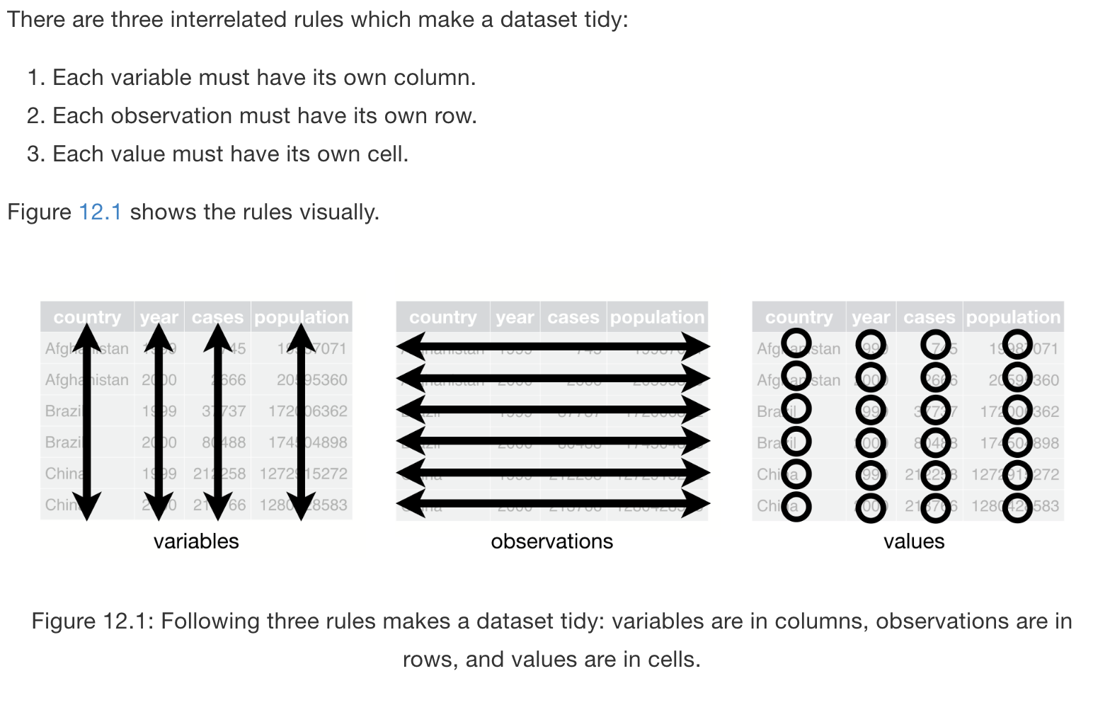
Principles of tidy data

7.8.1 Wide and long dataformats

We won't go into tidying data too much today, but we will look at one common phenomenon, when repeated measures are presented in a dataframe in the 'wide' format, that should be in the 'long' format. This might sound a bit funky, so let's look at an example.

This would be a reasonable dataset to encounter, in which for five individuals there are three measurements, one in year1, one in year2, and one in year3:

wide <- data.frame(
    ID = c(1, 2, 3, 4, 5),
    Age = c(22, 19, 35, 28, 42),
    Year1 = c(10, 2, 1, 9, 5),
    Year2 = c(9, 4, 6, 6, 1),
    Year3 = c(5, 6, 2, 7, 6)
  )
wide

##   ID Age Year1 Year2 Year3
## 1  1  22    10     9     5
## 2  2  19     2     4     6
## 3  3  35     1     6     2
## 4  4  28     9     6     7
## 5  5  42     5     1     6

While this dataframe looks sensible enough, it isn't "tidy". This is because Year1 and Year2 are not really names of variables but values of a variable (value 1, 2, and 3 from variable year). We can quite easily fix this with the help of the pivot_longer() function. To be able to use this function, we will need to install and call upon the tidyr package.

# install.packages("tidyr")
library(tidyr)

7.8.1.1 pivot_longer()

The pivot_longer function expects a dataframe and it expects you mention the names of the variables that need to be ‘elongated’ via cols. It also asks you to name a new column (that will include the names of variables you specified in cols via "names_to", and it asks you to name a new column in which the values of the columns in cols were stored via “values_to”. Let's try to use the function:

long <- pivot_longer(wide, cols = c(Year1, Year2, Year3), 
                     names_to = "Year", values_to = "Score")
long

## # A tibble: 15 × 4
##       ID   Age Year  Score
##    <dbl> <dbl> <chr> <dbl>
##  1     1    22 Year1    10
##  2     1    22 Year2     9
##  3     1    22 Year3     5
##  4     2    19 Year1     2
##  5     2    19 Year2     4
##  6     2    19 Year3     6
##  7     3    35 Year1     1
##  8     3    35 Year2     6
##  9     3    35 Year3     2
## 10     4    28 Year1     9
## 11     4    28 Year2     6
## 12     4    28 Year3     7
## 13     5    42 Year1     5
## 14     5    42 Year2     1
## 15     5    42 Year3     6

We went from a "wide"” to a "long"” format, because we have reduced the number of columns (we have reduced the width), but we have increased the number of rows (we have increased the height/length)! Although the long dataframe doesn't look much more intuitive than the wide format in this case, R deals with the long format much better. As an example, only with the long format are we able to create this graph instantly:

ggplot(long, aes(x = Year, y = Score, group = ID)) + 
  geom_line(colour = "grey") +
  geom_point() +
  theme_bw()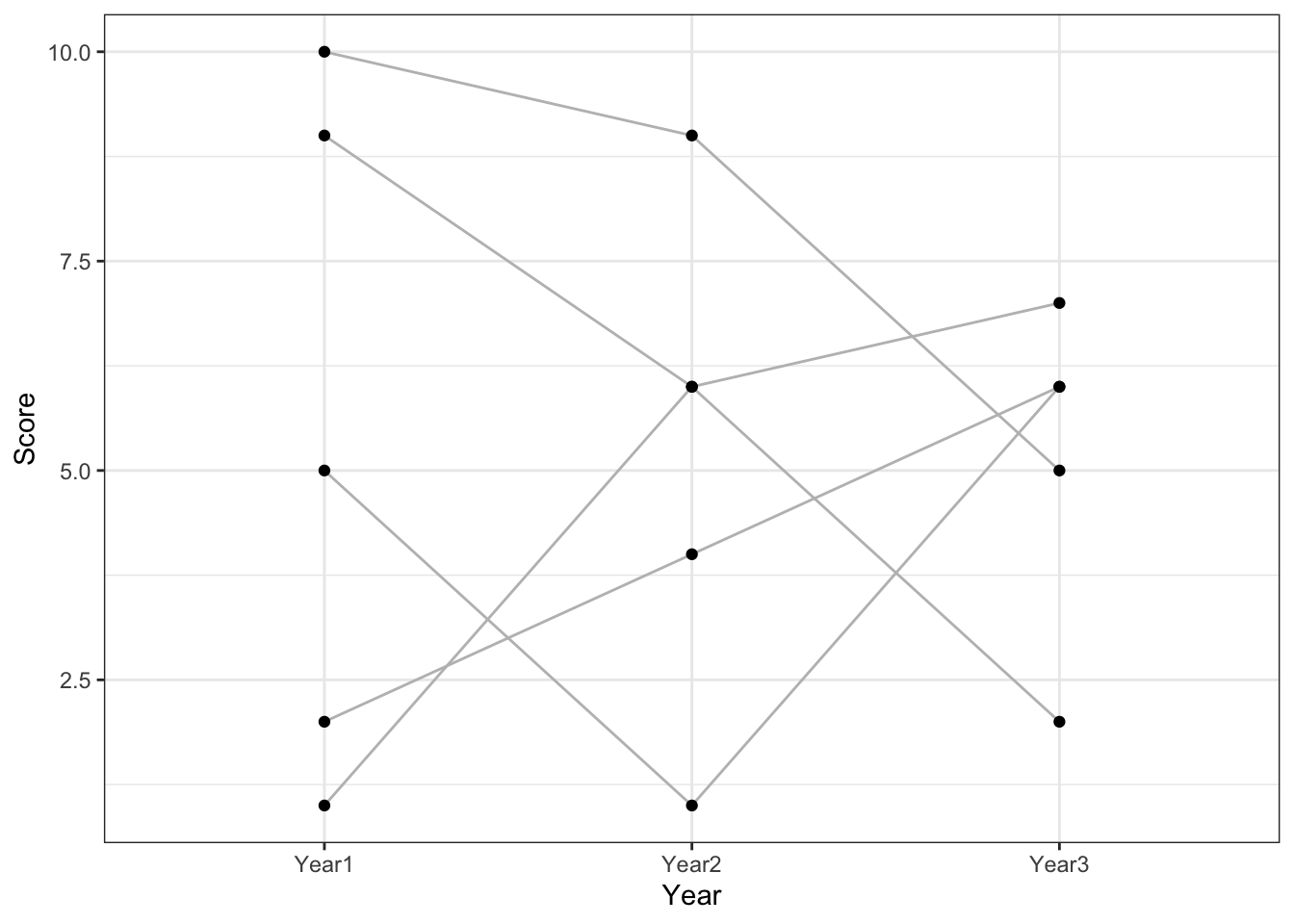

7.9 Assignments

1. From the mpg-dataset that is stored within df, select only the displ, year, and class variables. Use the pipe (%>%)!

2. Select all cases for the year 2008. Use the pipe (%>%)!

3. Create a mean and standard deviation for the displ-variable for the different classes of cars (the class variable). Remember, use the group_by and summarise function. Use the pipe (%>%)!

4. Put all the above actions into one long “pipe”!

7.10 Further reading

R for Data Science’s chapter on transforming data: http://r4ds.had.co.nz/transform.html. RStudio’s cheatshees are also very helpful! See the “Data Transformation Cheat Sheet” on https://www.rstudio.com/resources/cheatsheets/.

7.11 References

Wickham, Hadley. 2017. Tidyverse: Easily Install and Load the ‘Tidyverse’. https://CRAN.R-project.org/package=tidyverse.