Chapter 20 Colours

Of course, we can also change the colours in our graphs. We can make use of existing colour-sets from other packages, or we can specify our own colours.

20.1 Specifying your own colours

How to specify your own colour depends on what you have used for colouring. Let’s see what I mean here:

ggplot(mpg, aes(x=cty, colour=drv)) + geom_density()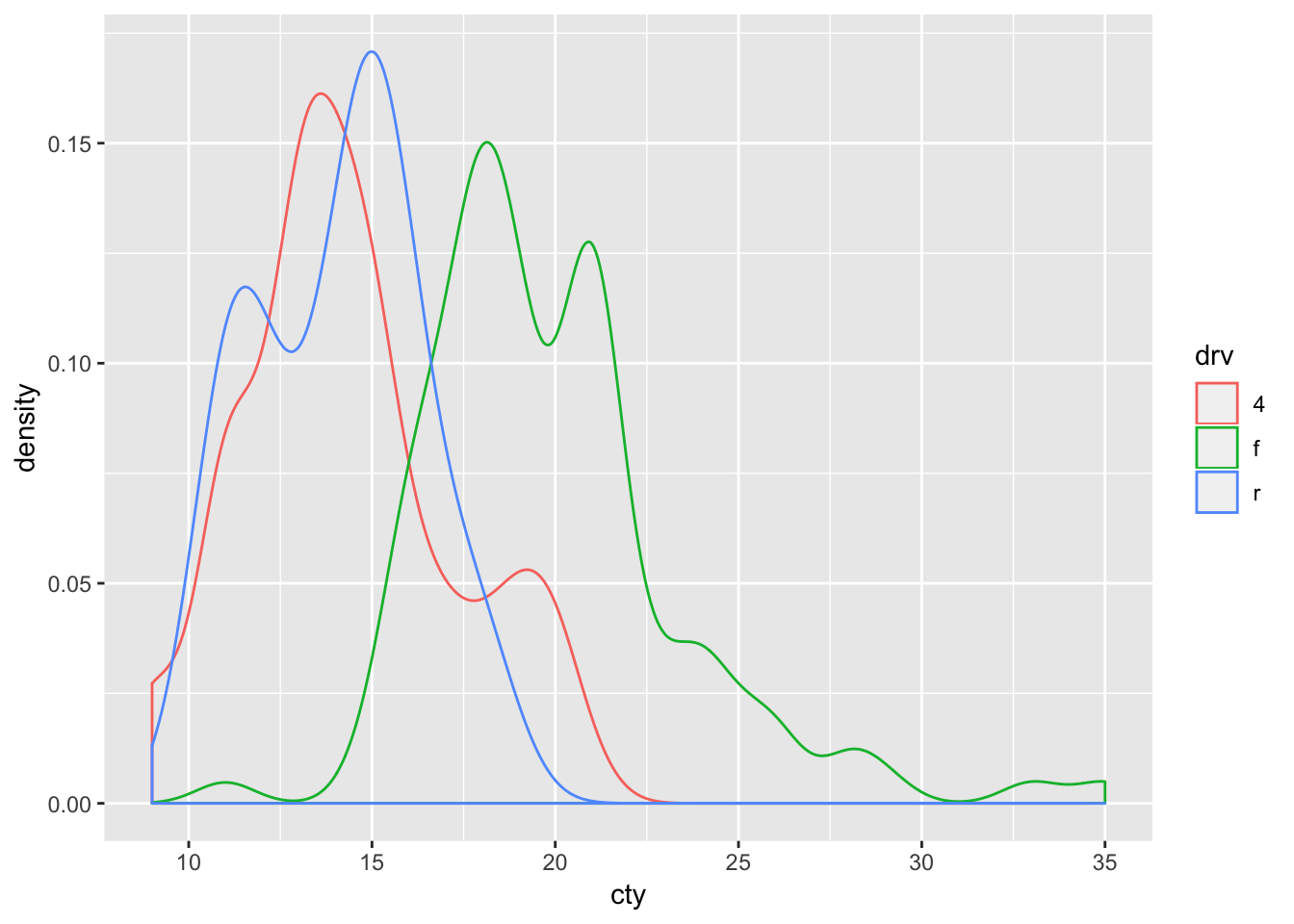

Here we have specified a ‘colour’ aesthetic. What if we want to use different colours? We can do this by using the scale functions:

ggplot(mpg, aes(x=cty, colour=drv)) + geom_density() +
  scale_colour_manual(values = c("4" = "lightblue", "f" = "yellow", "r" = "red"))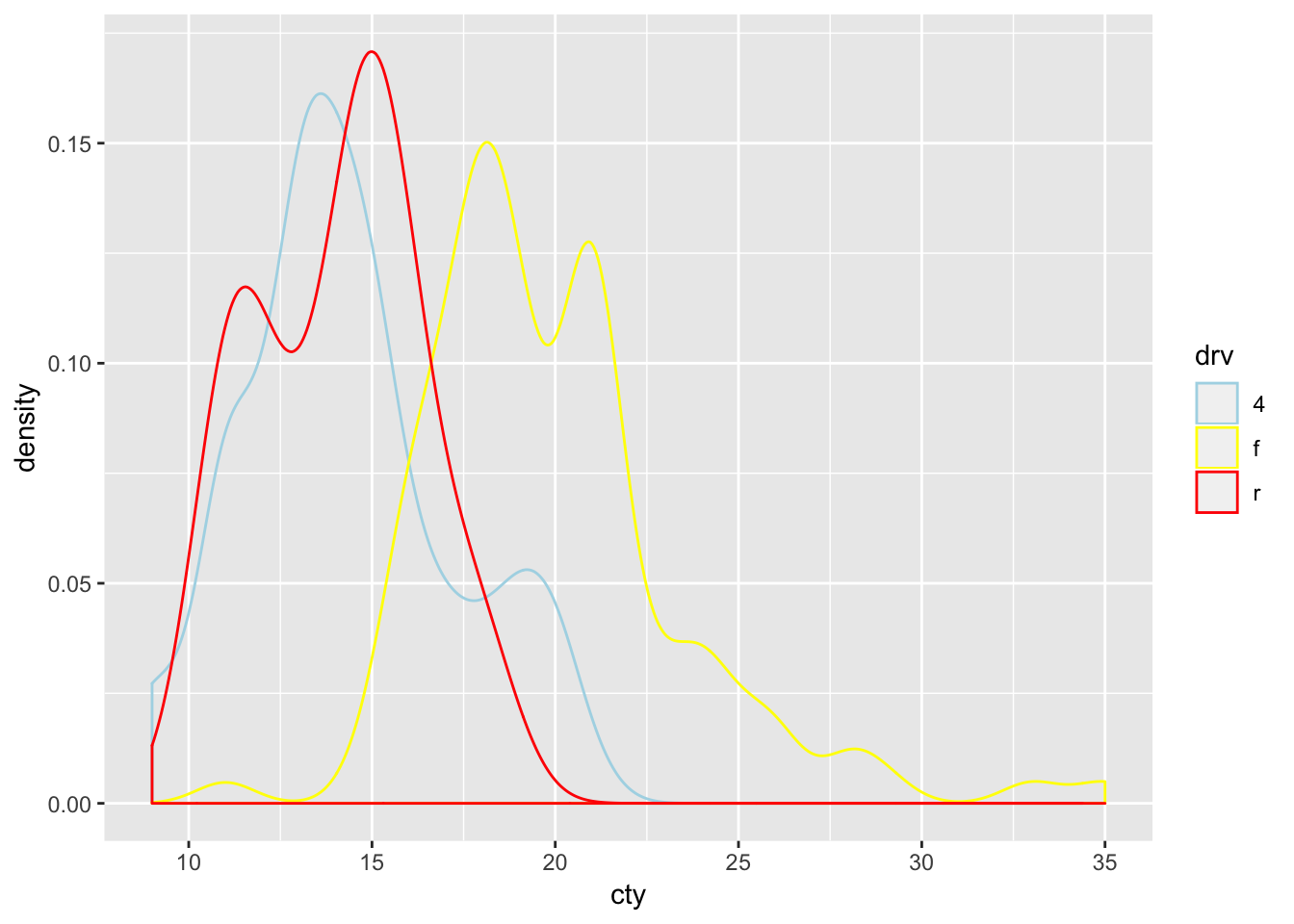

Well that certainly isn’t an improvement (do note that the colours that come with ggplot are certainly not randomly picked but are chosen for maximum discrimination between the colours). For names of other colours, see: http://sape.inf.usi.ch/quick-reference/ggplot2/colour and http://www.cookbook-r.com/Graphs/Colors_(ggplot2)/.

For this density plot, specifying fill is probably a bit nicer than specifying colour, so let’s try that:

ggplot(mpg, aes(x=cty, fill=drv)) + geom_density()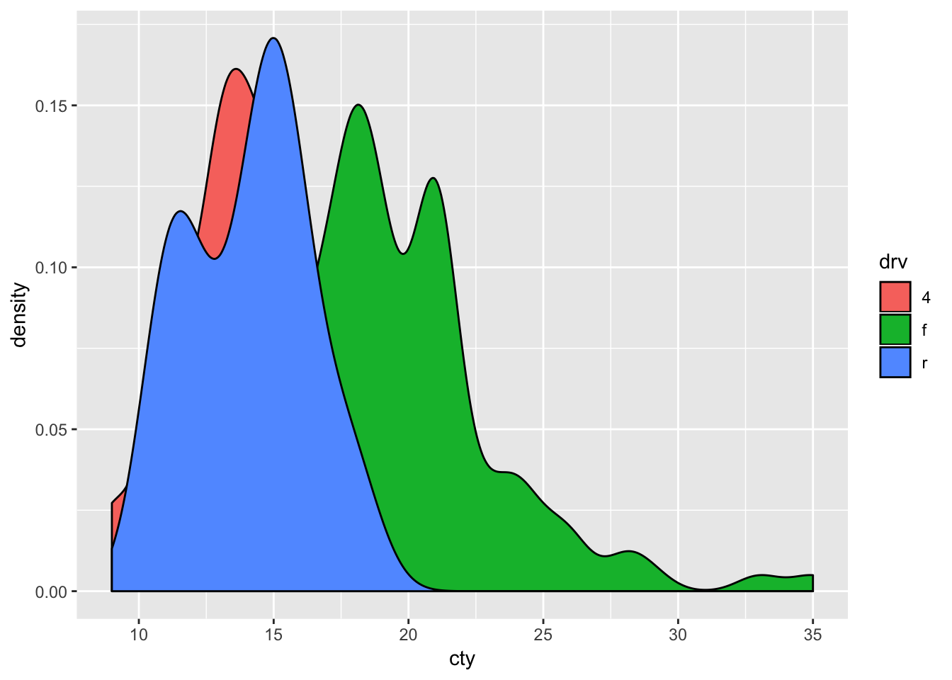 

And let’s change the colours with some newly chosen values

ggplot(mpg, aes(x=cty, fill=drv)) + geom_density()  +
  scale_colour_manual(values = c("4" = "magenta4", "f" = "cornflowerblue", "r" = "hotpink4"))

Hhhmm, that didn’t work. Why not? Because we have used scale_colour_manual despite the fact that we didn’t use colour! We should have used scale_fill_manual because we used fill

ggplot(mpg, aes(x=cty, fill=drv)) + geom_density()  +
  scale_fill_manual(values = c("4" = "magenta4", "f" = "cornflowerblue", "r" = "hotpink4"))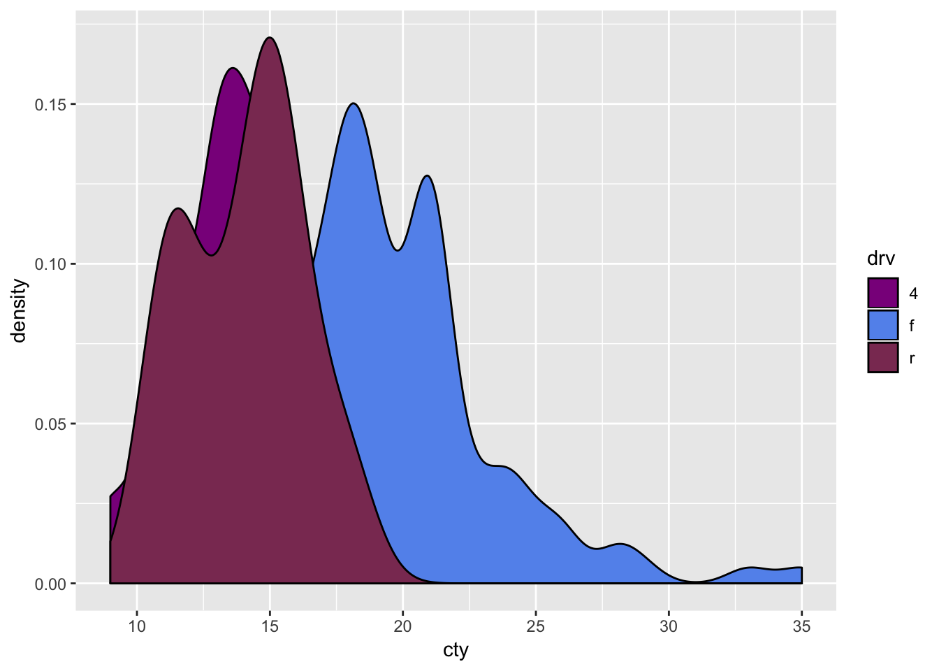

The above examples are useful when mapping colours to specific values. But sometimes we are using a gradient in colouring, for example:

ggplot(mpg, aes(x=cty, y=hwy, colour=displ)) + geom_point()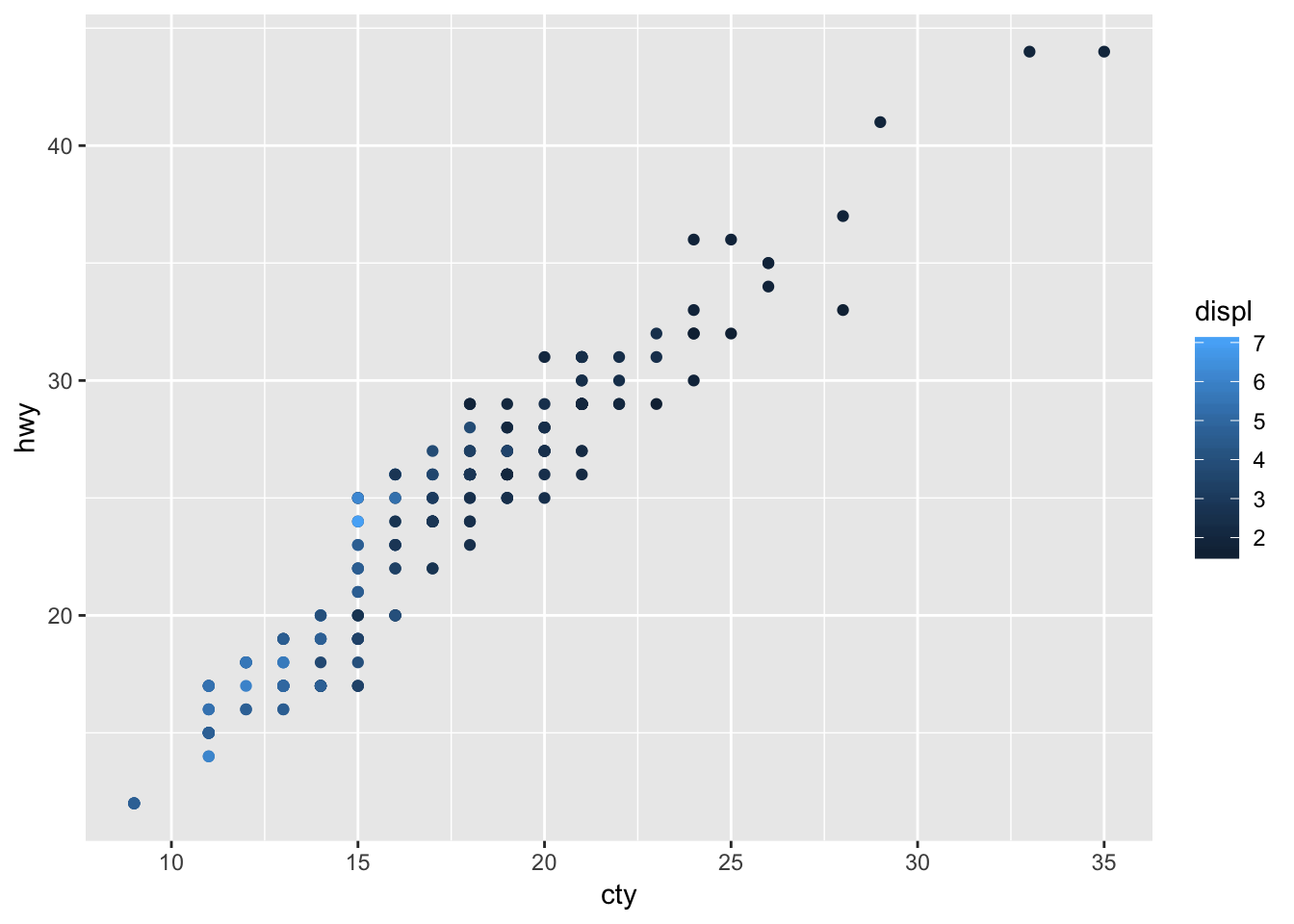 

We can also change the colours in this case, but a little bit differently:

ggplot(mpg, aes(x=cty, y=hwy, colour=displ)) + geom_point() + 
  scale_colour_gradient(low = 'blue', high = 'yellow')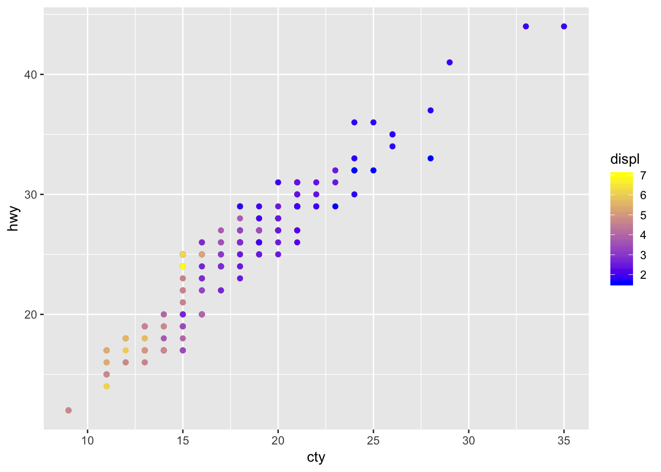

Another example:

ggplot(mpg, aes(x=cty, y=hwy, colour=displ)) + geom_point() + 
  scale_colour_gradient2(low = 'blue', mid = 'white', high = 'red', midpoint=4.5)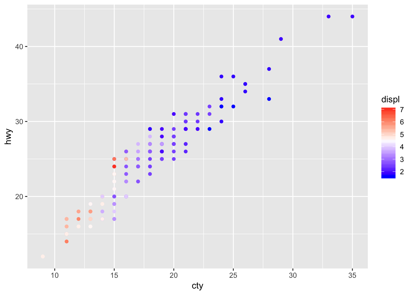

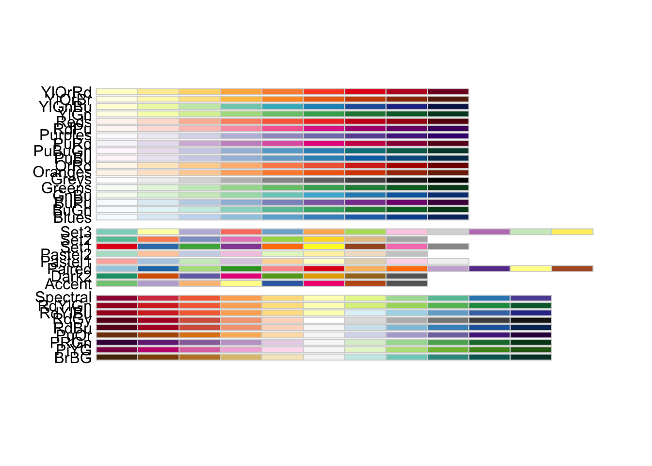
20.2 Existing colour sets

We can also make use of colour sets (or palettes) from other packages. Visually gifted people have chosen the palettes, and they can look very good:

# install.packages("RColorBrewer")
library(RColorBrewer)

ggplot(mpg, aes(x=cty, fill=class)) + geom_density()  +
  scale_fill_brewer(palette ="Set2")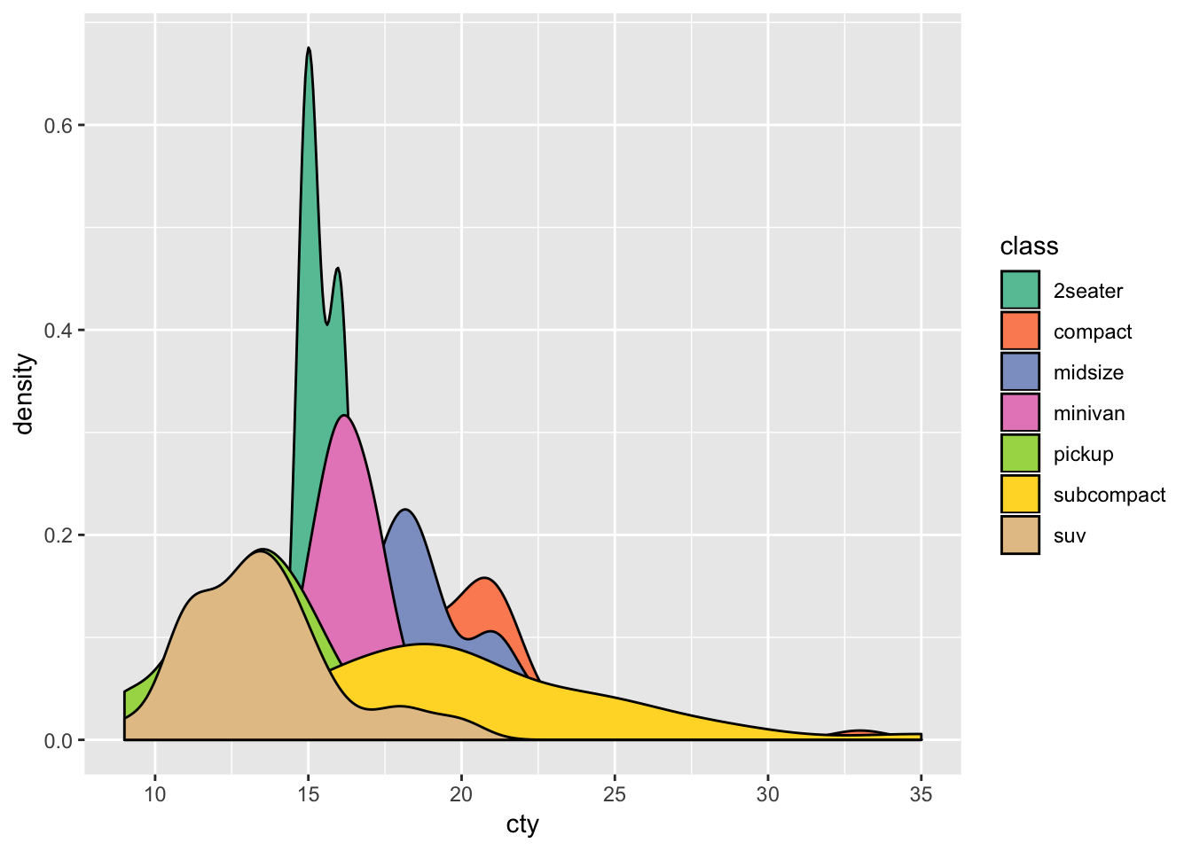

To see the different palettes on offer, use:

display.brewer.all()