Chapter 9 Distribution of a single variable
Typically a first step when analyzing data, is checking the distributions of the variables given their central role in deciding which analysis strategy to follow. We’ll look at some ways to do this, while at the same time changing some elements of the graphs that we get.
Two popular ways of showing a distribution are histograms and density plots; both give good ideas about the shape of the distribution.
9.1 Histogram
Making histograms is rather straightforward in ggplot, because there is a seperate “geom” for it, namely geom_histogram. Let’s make a histogram of the mileage per galon of fuel for the cars in the “mpg” dataset.
ggplot(mpg, aes(x=cty)) + geom_histogram()## `stat_bin()` using `bins = 30`. Pick better value with `binwidth`.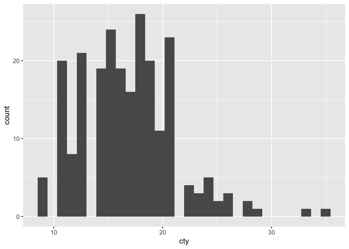
We have a histogram!
What does the histogram tell us?
Although the graph is fine, R tells us that “stat_bin() using bins = 30. Pick better value with binwidth”. To understand this a bit better, we must realize that a histogram counts the occurrences of particular values of the variable. For this, it makes use of “bins”, ranges of values. For instance, if we would choose a “binwidth” of 5, this would mean that the first bin equals 0-4, the second bin equals 5-9, et cetera. Choosing a binwidth that is too large or too small will result in somewhat funky histograms as we’ll see below.
Now let’s try and choose a different binwidth; R already gives us a hint as to how: by specifying binwidth:
ggplot(mpg, aes(x=cty)) + geom_histogram(binwidth=1)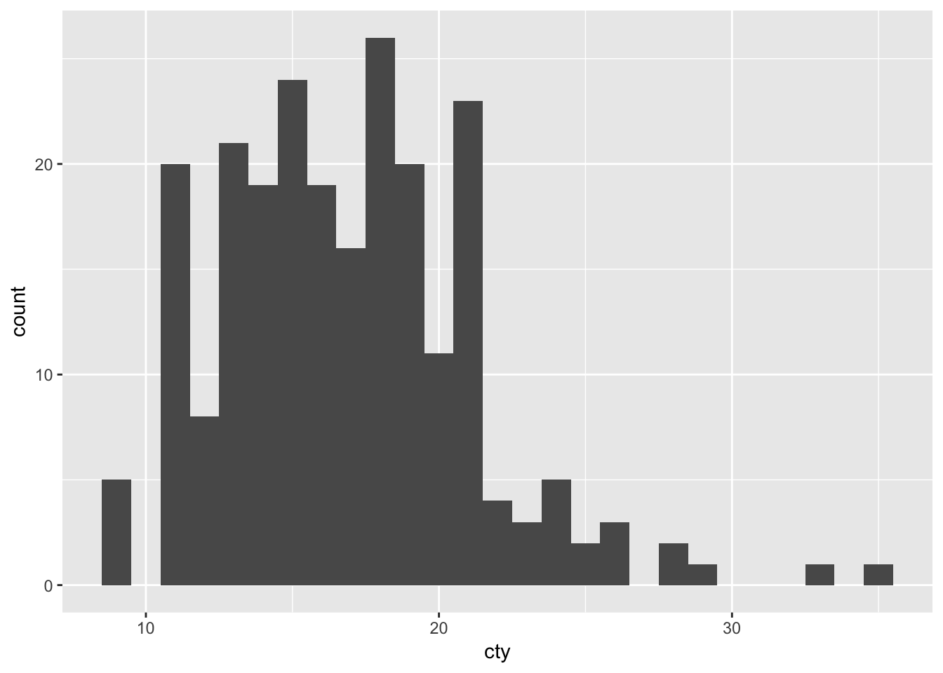
This graph resembles the previous one, but isn’t identical!
Let’s try other binwidths:
ggplot(mpg, aes(x=cty)) + geom_histogram(binwidth=5)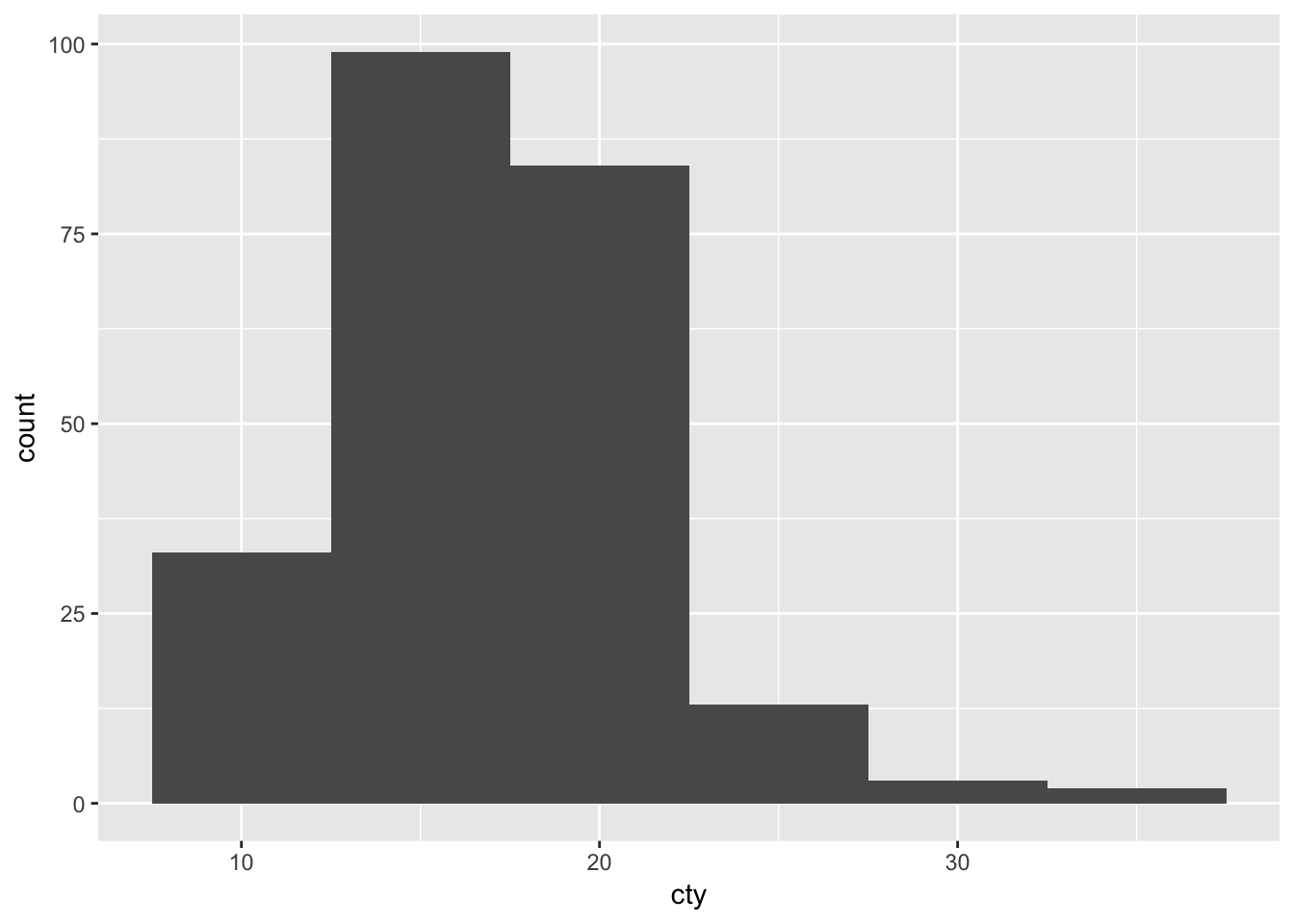
And another one:
ggplot(mpg, aes(x=cty)) + geom_histogram(binwidth=0.1)
What’s going on here?
Create a histogram of the variable ‘displ’ in the mpg-dataset [‘displ’ refers to the engine displacement, in litres]. What is a sensible binwidth?
Create a histogram of the variable ‘year’ in the mpg-dataset [‘year’ refers to the year that the model came out]. What can you conclude from this graph?
Now, what happens when we specify a y-variable?
ggplot(mpg, aes(x=cty, y=drv)) + geom_histogram(binwidth=1)## Error: stat_bin() must not be used with a y aesthetic.R gives an error. Maybe this is also not very surprising; what is the y-variable supposed to do? A histogram is a rather specific type of graph where the numbers (or percentages) of occurences are put on the y-axis from the variable that is chosen as x-variable. So the y is already defined (more or less), and our specification doesn’t work. The function geom_histogram() does some of the computing for us, with the function stat_bin() that apparently cannot be used with a y-variable.
And what happens if we try to make a histogram of a non-continuous variable (in this case the model of the car)?
ggplot(mpg, aes(x=model)) + geom_histogram(binwidth=1, colour="orange")## Error: StatBin requires a continuous x variable the x variable is discrete. Perhaps you want stat="count"?Clearly the geom_histogram() function doesn’t like it when the x variable is not continuous, and a plot is not provided. It give us some suggestion how to resolve it, but we won’t go into that. If you want help in R, you can type ?geom_histogram which will give you some information. I find the information provided by R rather difficult to read, so I’ll typically use google. The ‘official’ ggplot-pages are incredibly helpful: http://ggplot2.tidyverse.org/reference/geom_histogram.html. See also Chapter 22.
9.1.1 Tweaking the histogram
Now let’s quickly alter some of the features in the graph. We’ll learn more about this in later chapters, but it’s good to get an idea of what can be done.
We can easily change the colour of the bars. Let’s make them orange, because why not:
ggplot(mpg, aes(x=cty)) + geom_histogram(binwidth=1, colour="orange")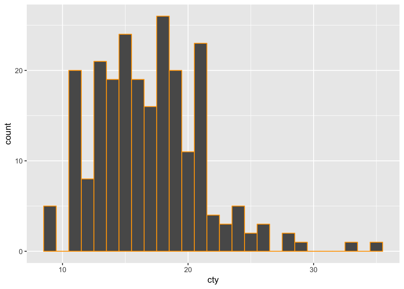
It worked! Sort of. We’ve coloured the outer sides of the bars, but the filling within is still black. So let’s change the filling as well (with the rather intuitive fill=), and choose the colour blue:
ggplot(mpg, aes(x=cty)) +
  geom_histogram(binwidth=1, colour="orange", fill="blue")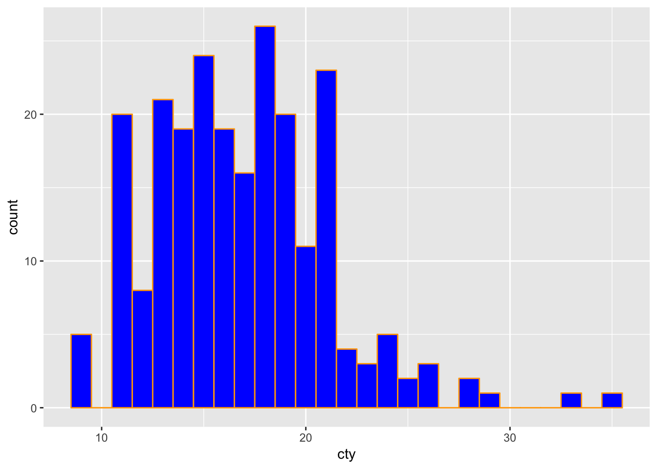
What an ugly histogram!
If we want no fill, we will have to define the fill as NA (which is the value of missing within R; NA stands for Not Available):
ggplot(mpg, aes(x=cty)) + geom_histogram(binwidth=1, colour="orange", fill=NA)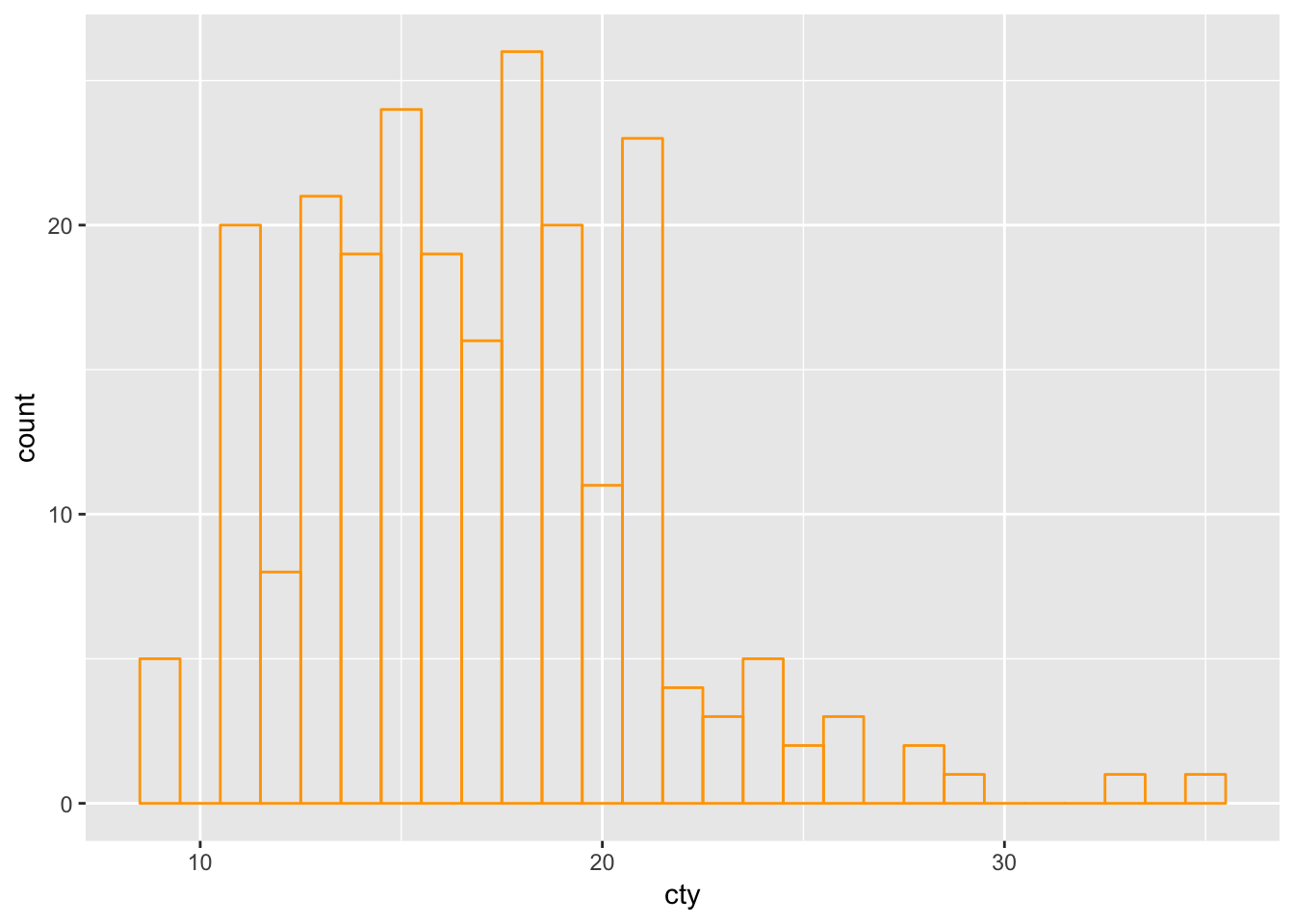
We can also remove the border in a similar way:
ggplot(mpg, aes(x=cty)) + geom_histogram(binwidth=1, colour=NA, fill="blue")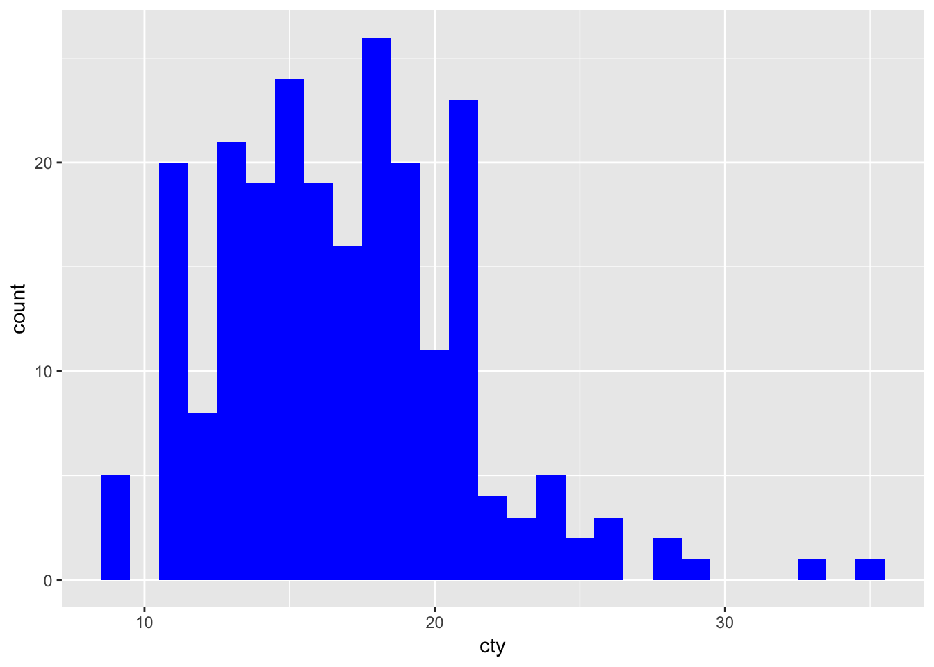
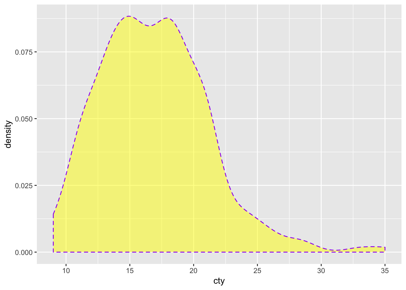
The ggplot-cheatsheet tells us some of the other appearence-features we can in a histogram: “alpha, color, fill, linetype, size” (“weight” can be used to weigh the cases). Let’s try them all:
ggplot(mpg, aes(x=cty)) +
  geom_histogram(binwidth=1,
                 colour="purple", # Make the borders purple
                 fill="yellow", # Make the fill of the bars yellow
                 alpha=0.5, # Make the fill see through 50%
                 linetype="dashed", # Make the borders dashed
                 size=0.5 # Make the size of the borders smaller
  )
9.2 Density plot
Another way of plotting a distribution of a single variable, is to make use of density plots. This is similar to a histogram, except that the distribution is based on a smoothening-function:
ggplot(mpg, aes(x=cty)) + geom_density()
Not quite as informative as the histogram, but density plots can be handy when comparing distributions (as we’ll see shortly).
9.2.1 Tweaking the density plot
We can tweak some of the features in ways that are very similar to the histogram.
The ggplot-cheatsheet tells us some of the other appearence-features we can use with a density plot: “alpha, color, fill, linetype, size” (“weight” can be used to weigh the cases). Let’s try them all:
ggplot(mpg, aes(x=cty)) +
  geom_density(colour="purple", # Make the borders purple
               fill="yellow", # Make the fill of the bars yellow
               alpha=0.5, # Make the fill see through 50%
               linetype="dashed", # Make the borders dashed
               size=0.5 # Make the size of the borders smaller
  )
Create a new density plot of the variable “cty”; remove the fill-colour, and choose as linetype “dotted”; change the size to any value you’d like. [is alpha still sensible?]
For more info, see http://ggplot2.tidyverse.org/reference/geom_density.html. We’ll also see more density plots when we address the (beautiful) violin plots.
9.3 The frequency polygon
Two other ways of visualizing a distribution are a frequency polygon, and a dotplot. Both are less often used than histograms and density plots, but they have their use.
To get a frequency polygon, use:
ggplot(mpg, aes(x=cty)) + geom_freqpoly(binwidth=1)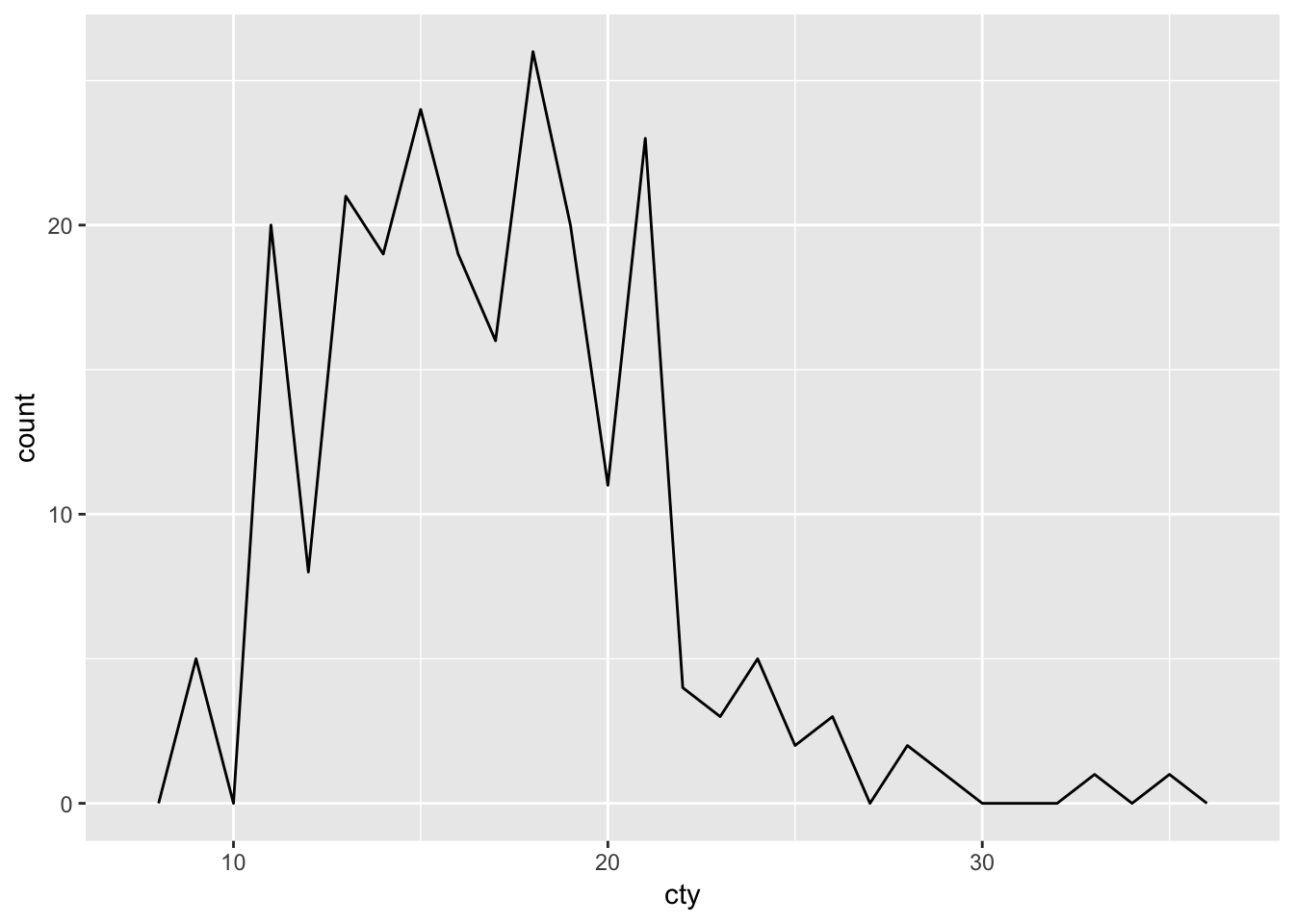 The frequency polygon is very similar to the histogram in that the information in the graph is similar (and the calculations are identical and need a “binwidth”).
When do you think a frequency polygon is preferred over histograms and density plots?
For more information on frequency polygons, visit http://ggplot2.tidyverse.org/reference/geom_histogram.html.
9.4 The dotplot
To get a dotplot, use:
ggplot(mpg, aes(x=cty)) + geom_dotplot(binwidth=0.5)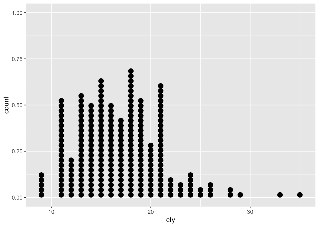
Every dot is a case, and dots within an ‘bin’ are stacked on top of each other. This is very similar a histogram in this form. An alternative way of stacking the dots is:
ggplot(mpg, aes(x=cty)) + geom_dotplot(binwidth=0.5, stackdir = "center")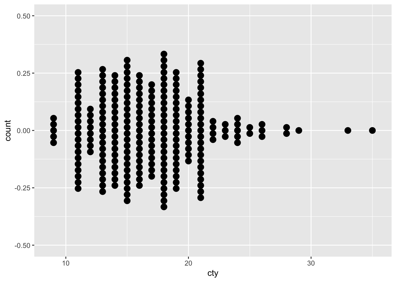
The y-axis is not very helpful (in both cases; because it depends on the binning algorithm and some features that we can pass to the geom_dotplot function), so we can supress it if we want to (for more info on changing the scales/axes, see 16):
ggplot(mpg, aes(x=cty)) + geom_dotplot(binwidth=0.5, stackdir = "center") +
  scale_y_continuous(name = NULL, breaks = NULL)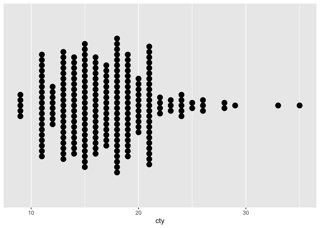
For more information on dotplots, see http://ggplot2.tidyverse.org/reference/geom_dotplot.html