Chapter 17 The legend

Sometimes we want to adapt the legend a bit. Here we’ll see some popular options:

17.1 Removing the legend.

ggplot(mpg, aes(x=hwy, y=cty, colour=drv)) + geom_point() + 
  guides(colour=FALSE)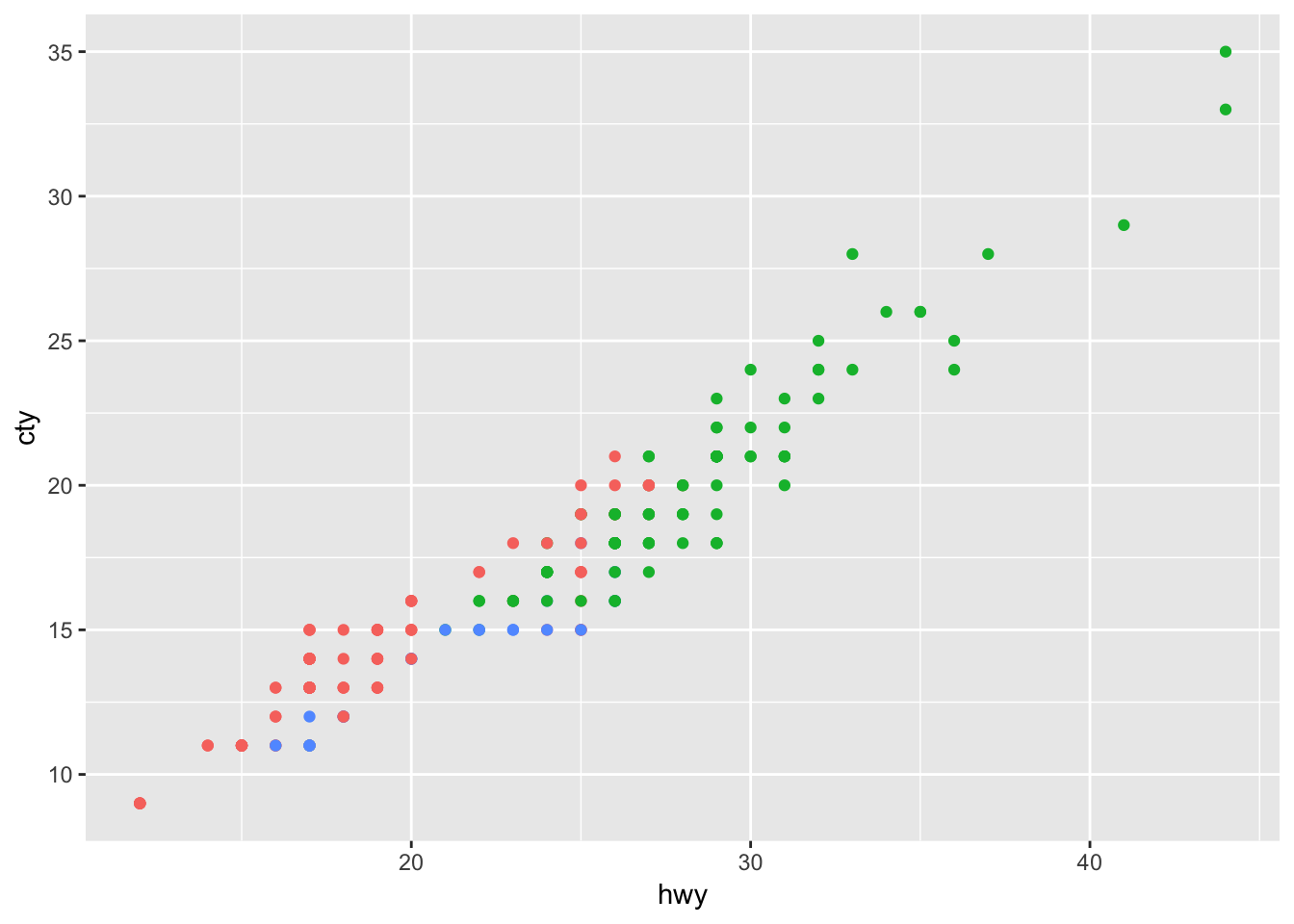

17.2 Changing location of legend

ggplot(mpg, aes(x=hwy, y=cty, colour=drv)) + geom_point() + 
  theme(legend.position="top") # options: top, left, right, bottom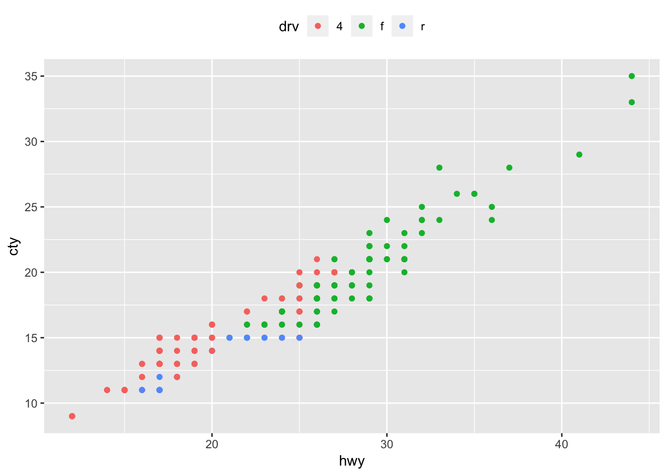

You can also specify a position with two numbers between 0 and 1. The first number means the position on the x-axis, 0 means all the way at the start of the x-axis (i.e., to the left), 0.5 means halfway, and 1 means all the way at the end of the x-axis. The second number does the same for the y-axis, where 0 is the lowest value of the y-axis, and 1 the highest. Setting the legend to c(0.5, 0.5) means that the legend will be placed right in the middle (with the center of the legend exactly on the middle point of the graph!):

ggplot(mpg, aes(x=hwy, y=cty, colour=drv)) + geom_point() + 
  theme(legend.position=c(0.5,0.5))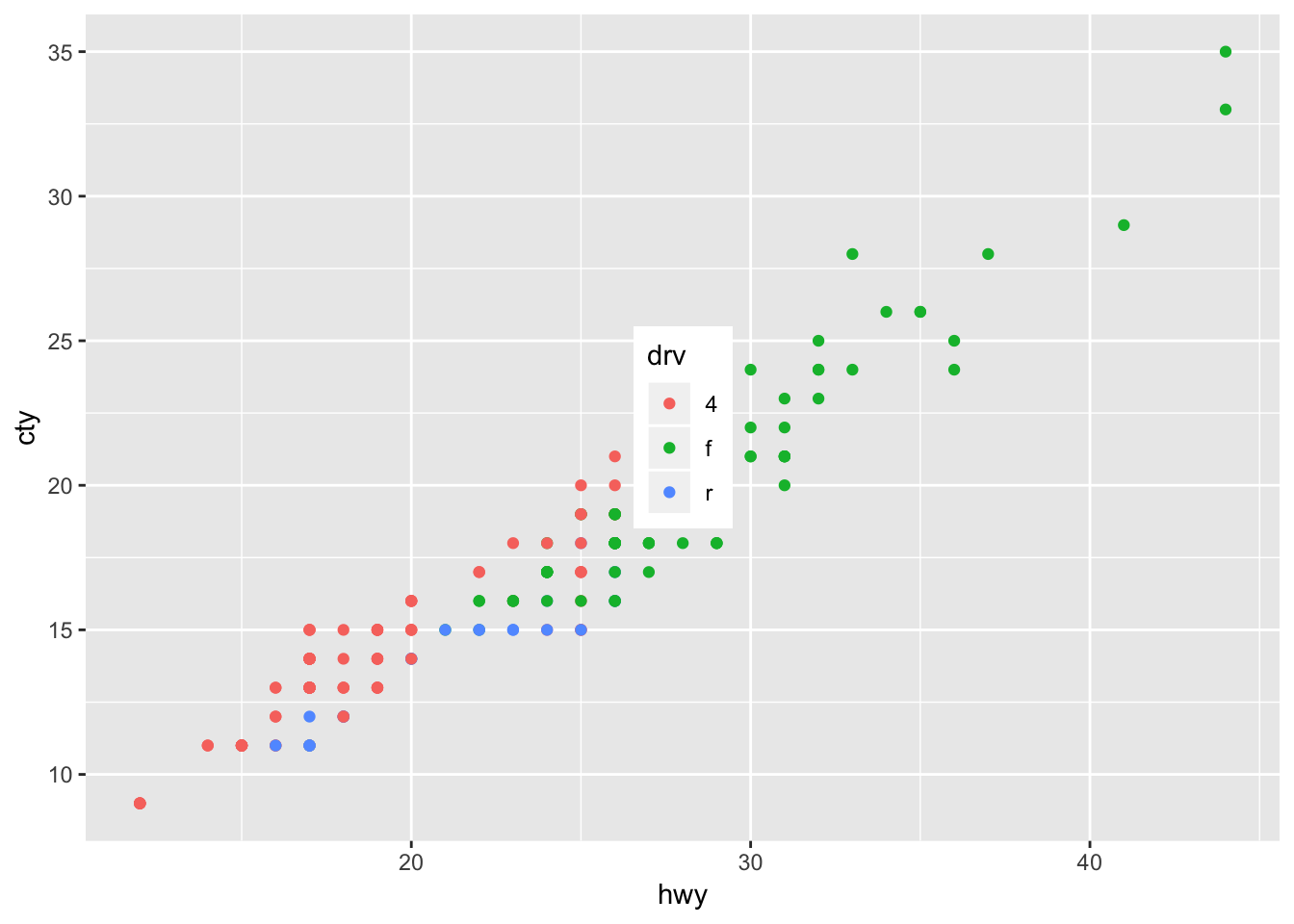 

Another option:

ggplot(mpg, aes(x=hwy, y=cty, colour=drv)) + geom_point() + 
  theme(legend.position=c(0.1,0.8))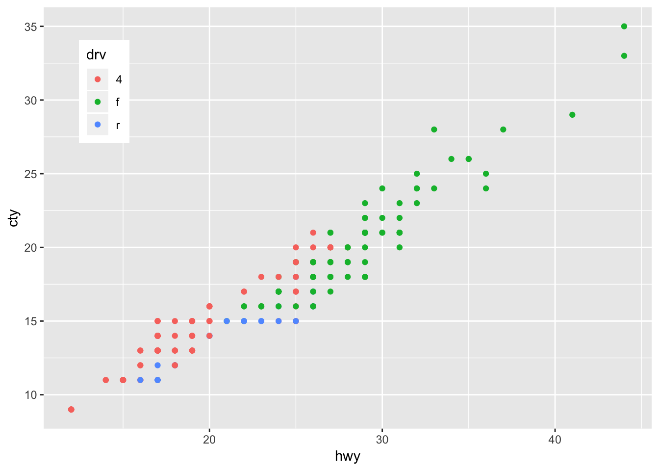 

We’ve seen we can change the position of the legend by using the legend.position function. Often it is helpful to also use legend.justification. For instance, let’s try and place the legend in the right bottom corner:

ggplot(mpg, aes(x=hwy, y=cty, colour=drv)) + geom_point() + 
  theme(legend.position=c(1,0))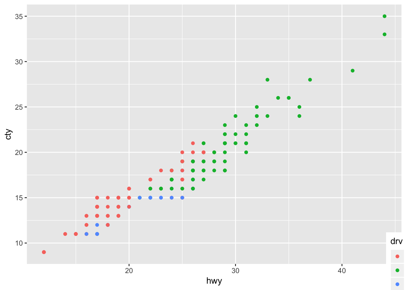 

Why does this happen?

The centre of the legend is placed on the designated location. We can change this by using the legend.justification. Again we specify two numbers. One number specifies what should happen with the boundaries of the legend in the horizontal dimension; a 0 indicates that the left boundary will be set at the x-position specified (the legend will be shifted to the rightt), a 1 means that the right boundary will be set at the x-position specified (the legend will be shifted to the left). The second number does the same for the vertical dimension, where a 0 shifts the legend upwards, and a 1 downwards.

ggplot(mpg, aes(x=hwy, y=cty, colour=drv)) + geom_point() + 
  theme(legend.position=c(1,0), legend.justification=c(1,0))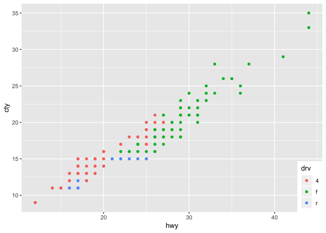 

Play around with the legend.position and legend.justification; do you see the pattern?

17.3 Changing order in legend

You’ll find you often need this, so it is important to see how to do this:

ggplot(mpg, aes(x=hwy, y=cty, colour=drv)) + geom_point() + 
  scale_colour_discrete(limits=c("f", "r", "4"))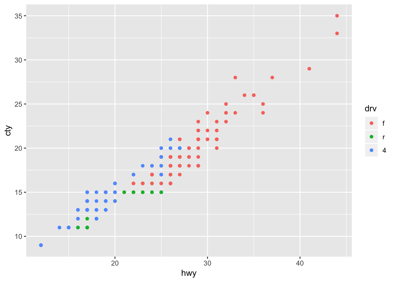 

17.4 Changing features of legend

We can also change some features of the legend itself:

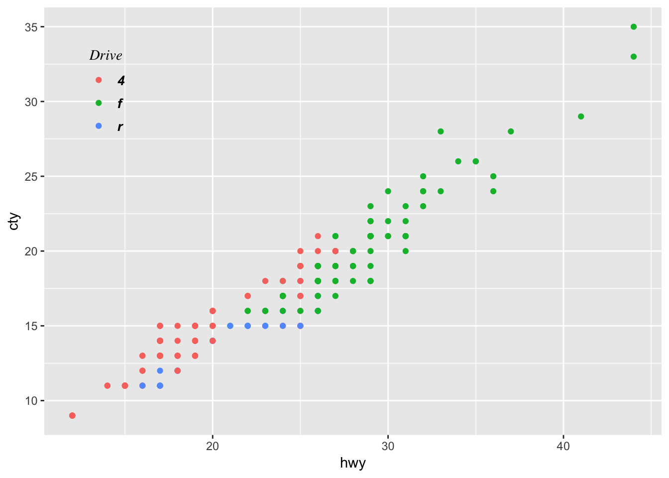
ggplot(mpg, aes(x=hwy, y=cty, colour=drv)) + geom_point() + 
  labs(colour="Drive") +
  theme(legend.position=c(0.1,0.8),
        legend.background=element_blank(),
        legend.key=element_blank(),
        legend.title = element_text(family ="serif", face="italic"),
        legend.title.align=0.5,
        legend.text = element_text(face="bold.italic", size=10))