Chapter 19 Themes
With the ‘theme’-argument (theme()) you can adjust (nearly) all appearence features of the graph. ggplot also provides some themes that can give you an impression of what is possible.
19.1 Standard themes
The standard themes of ggplot include: theme_bw, theme_gray, theme_dark, theme_classic, theme_minimal, theme_void
regular <- ggplot(mpg, aes(x=displ, y=cty, colour=drv)) + geom_point() + labs(title="No theme")
bw <- ggplot(mpg, aes(x=displ, y=cty, colour=drv)) + geom_point() + theme_bw() + labs(title="theme_bw")
gray <- ggplot(mpg, aes(x=displ, y=cty, colour=drv)) + geom_point() + theme_gray() + labs(title="theme_gray")
dark <- ggplot(mpg, aes(x=displ, y=cty, colour=drv)) + geom_point() + theme_dark() + labs(title="theme_dark")
classic <- ggplot(mpg, aes(x=displ, y=cty, colour=drv)) + geom_point() + theme_classic() + labs(title="theme_classic")
minimal <- ggplot(mpg, aes(x=displ, y=cty, colour=drv)) + geom_point() + theme_minimal() + labs(title="theme_minimal")
void <- ggplot(mpg, aes(x=displ, y=cty, colour=drv)) + geom_point() + theme_void() + labs(title="theme_void")
Showing multiple figures at once takes some effort:
# install.packages("gridExtra")
library(gridExtra)
grid.arrange(regular,bw, gray, dark, classic, minimal, void,  ncol=3)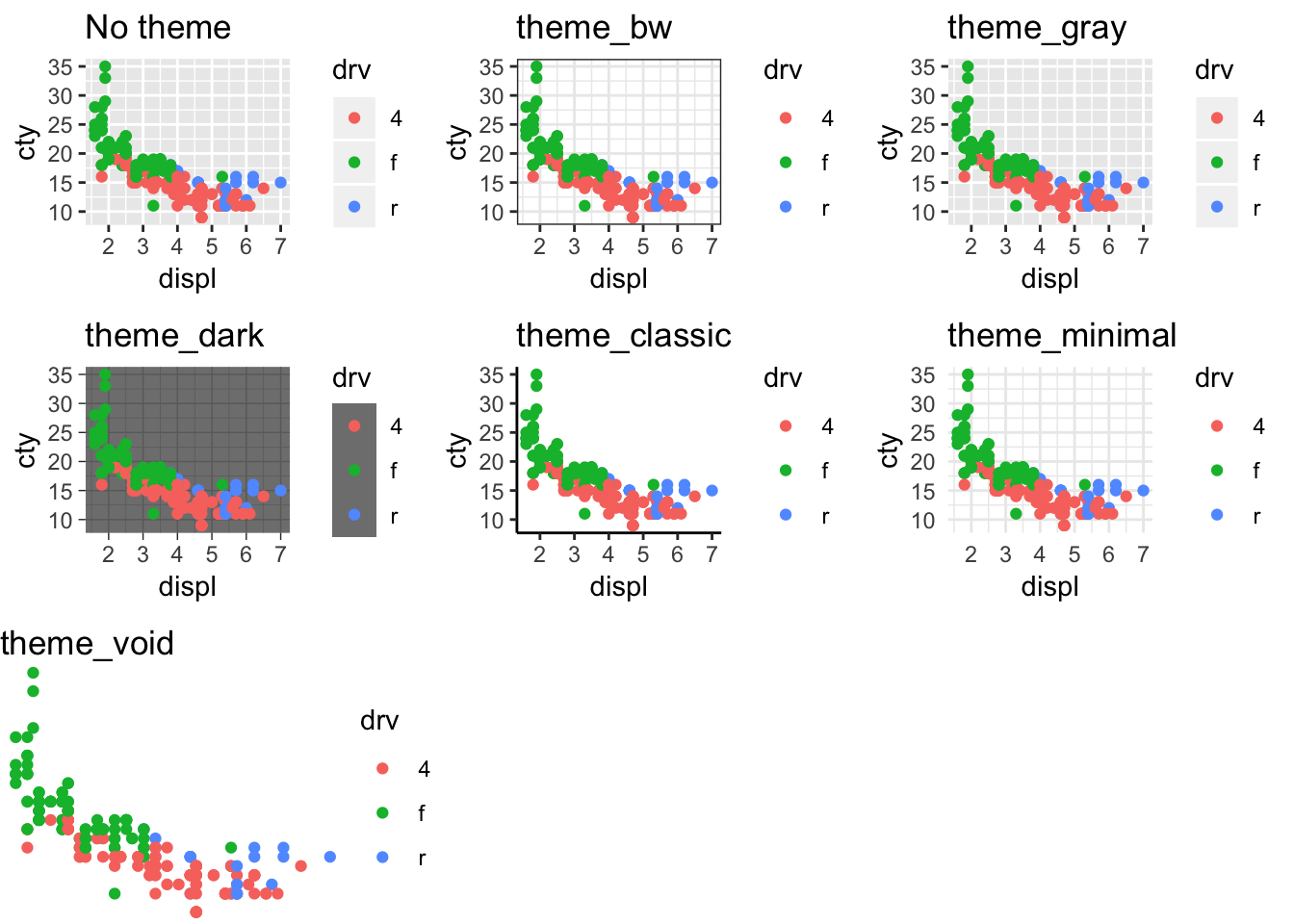
19.2 Customized themes
You can really change a lot of features from the graph, allowing you to create the exact graph you had in mind. Look at all the options within theme (plus an explanation of each aspect here: http://ggplot2.tidyverse.org/reference/theme.html)
theme(line, rect, text, title, aspect.ratio, axis.title, axis.title.x,
  axis.title.x.top, axis.title.y, axis.title.y.right, axis.text, axis.text.x,
  axis.text.x.top, axis.text.y, axis.text.y.right, axis.ticks, axis.ticks.x,
  axis.ticks.y, axis.ticks.length, axis.line, axis.line.x, axis.line.y,
  legend.background, legend.margin, legend.spacing, legend.spacing.x,
  legend.spacing.y, legend.key, legend.key.size, legend.key.height,
  legend.key.width, legend.text, legend.text.align, legend.title,
  legend.title.align, legend.position, legend.direction, legend.justification,
  legend.box, legend.box.just, legend.box.margin, legend.box.background,
  legend.box.spacing, panel.background, panel.border, panel.spacing,
  panel.spacing.x, panel.spacing.y, panel.grid, panel.grid.major,
  panel.grid.minor, panel.grid.major.x, panel.grid.major.y, panel.grid.minor.x,
  panel.grid.minor.y, panel.ontop, plot.background, plot.title, plot.subtitle,
  plot.caption, plot.margin, strip.background, strip.placement, strip.text,
  strip.text.x, strip.text.y, strip.switch.pad.grid, strip.switch.pad.wrap, ...,
  complete = FALSE, validate = TRUE)
Let’s change some features:
ggplot(mpg, aes(x=displ, y=cty, colour=drv)) + geom_point() +
  theme(axis.title = element_text(size =18, face="bold"),
        legend.position="top",
        plot.background = element_rect("grey"),
        panel.background = element_rect("white"),
        panel.grid.major = element_line(size=1, linetype="dashed", colour="darkgrey"),
        legend.background = element_rect(colour="orange", fill="green"))
What might be handy to realize is that you can also store your theme options and use them: Let’s change some features:
my_theme <- theme(axis.title = element_text(size =18, face="bold"),
        legend.position="top",
        plot.background = element_rect("grey"),
        panel.background = element_rect("white"),
        panel.grid.major = element_line(size=1, linetype="dashed", colour="darkgrey"),
        legend.background = element_rect(colour="orange", fill="green"))

ggplot(mpg, aes(x=displ, y=cty, colour=drv)) + geom_point() + my_theme
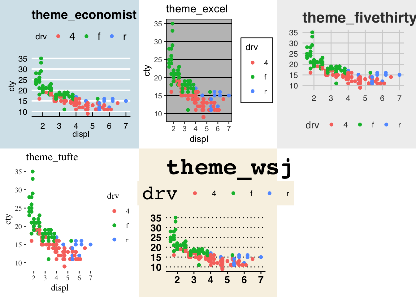
19.3 Other themes
We can also use themes that were made by others. For instance, by making use of the package ggthemes we can recreate graphs in the style of “The economist”, or, “Wall Street Journal”, or old awful excel graphs. Let’s see some cool examples:
# install.packages("ggthemes")
library(ggthemes)

econ <- ggplot(mpg, aes(x=displ, y=cty, colour=drv)) + geom_point() + theme_economist() + labs(title="theme_economist")
excel <- ggplot(mpg, aes(x=displ, y=cty, colour=drv)) + geom_point() + theme_excel() + labs(title="theme_excel")
fte <- ggplot(mpg, aes(x=displ, y=cty, colour=drv)) + geom_point() + theme_fivethirtyeight() + labs(title="theme_fivethirtyeightk")
tufte <- ggplot(mpg, aes(x=displ, y=cty, colour=drv)) + geom_point() + theme_tufte() + labs(title="theme_tufte")
wsj <- ggplot(mpg, aes(x=displ, y=cty, colour=drv)) + geom_point() + theme_wsj() + labs(title="theme_wsj")
grid.arrange(econ, excel, fte, tufte, wsj,  ncol=3)