Chapter 9 Do It Yourself
library(readr)
library(ggplot2)
library(ggraph)
library(igraph)
library(tidygraph)
library(tidyverse)
9.1 Eugenio Petrovich
Read-in data:
eugenio <- read_csv2("https://stulp.gmw.rug.nl/patio/Author_ackgees_homophily.csv")
head(eugenio)
## # A tibble: 6 × 6
## ID Sender Sender_gender Receiver Receiver_gender Weight
## <dbl> <chr> <chr> <chr> <chr> <dbl>
## 1 1 Sarah Moss female Sam Carter male 1
## 2 2 Sarah Moss female Keith DeRose male 1
## 3 3 Sarah Moss female Ben Holguin male 1
## 4 4 Sarah Moss female Ofra Magidor female 1
## 5 5 Sarah Moss female Daniel Rothschild male 1
## 6 6 Sarah Moss female Julia Staffel female 1The edge list and node attributes are combined. Let’s seperate them first.
eugenio_edges <- eugenio %>%
  select(Sender, Receiver, Weight) %>%
  rename(from = "Sender",
         to = "Receiver")
head(eugenio_edges)
## # A tibble: 6 × 3
## from to Weight
## <chr> <chr> <dbl>
## 1 Sarah Moss Sam Carter 1
## 2 Sarah Moss Keith DeRose 1
## 3 Sarah Moss Ben Holguin 1
## 4 Sarah Moss Ofra Magidor 1
## 5 Sarah Moss Daniel Rothschild 1
## 6 Sarah Moss Julia Staffel 1# number of unique names in sender + gender of sender
sender_unique <- eugenio %>%
select(Sender, Sender_gender) %>%
rename(person = "Sender",
gender = "Sender_gender") %>% # rename variable for combining datasets
unique() # select only unique rows
receiver_unique <- eugenio %>%
select(Receiver, Receiver_gender) %>%
rename(person = "Receiver",
gender = "Receiver_gender") %>% # rename variable for combining datasets
unique() # select only unique rows
eugenio_nodes <- bind_rows(sender_unique, receiver_unique) %>% unique()
head(eugenio_nodes)## # A tibble: 6 × 2
## person gender
## <chr> <chr>
## 1 Sarah Moss female
## 2 Colin Chamberlain male
## 3 Maegan Fairchild female
## 4 Ram Neta male
## 5 Matthew Mandelkern male
## 6 Jacob M. Nebel maleeugenio_nw <- tbl_graph(nodes = eugenio_nodes, edges = eugenio_edges, directed = TRUE)
eugenio_nw## # A tbl_graph: 5909 nodes and 18922 edges
## #
## # A directed multigraph with 27 components
## #
## # Node Data: 5,909 × 2 (active)
## person gender
## <chr> <chr>
## 1 Sarah Moss female
## 2 Colin Chamberlain male
## 3 Maegan Fairchild female
## 4 Ram Neta male
## 5 Matthew Mandelkern male
## 6 Jacob M. Nebel male
## # … with 5,903 more rows
## #
## # Edge Data: 18,922 × 3
## from to Weight
## <int> <int> <dbl>
## 1 1 1266 1
## 2 1 1267 1
## 3 1 1268 1
## # … with 18,919 more rowsLet’s calculate some clusters
eugenio_nw <- eugenio_nw %>%
  activate(nodes) %>%
  mutate(clusters = group_infomap()) %>%
  group_by(clusters) %>%
  mutate(cluster_size = n()) %>% # determine cluster size
  ungroup()
It takes llloooonnnnggggg, and the result is not too insightful.
ggraph(eugenio_nw, layout = "mds") +
  geom_edge_link(alpha = 0.1) +
  geom_node_point(aes(colour = factor(clusters)) )+
  theme_graph() +
  scale_colour_viridis_d() +
  theme(legend.position = "none")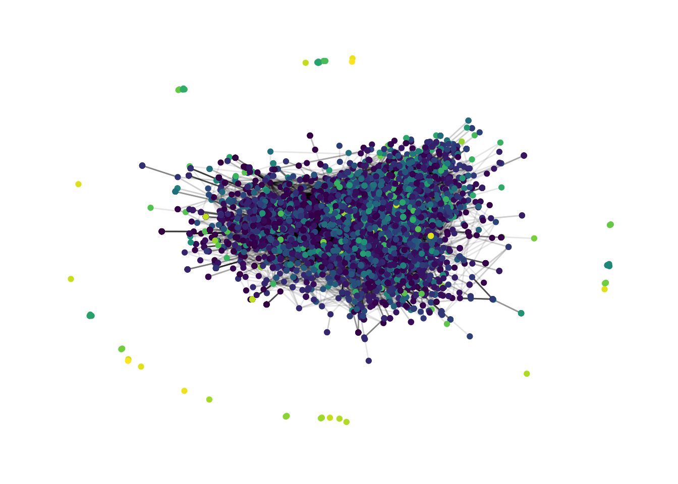
Because it takes so long, I decided to select only the two largest clusters.
# Retrieve 2 largest clusters
top_2 <- eugenio_nw %>%
  activate(nodes) %>%
  as_tibble() %>%
  arrange(desc(cluster_size)) %>%
  select(cluster_size) %>%
  unique() %>%
  slice(1:2) %>%
  pull(cluster_size)

# select tidygraph object with only two largest clusters
eugenio_nw_top2 <- eugenio_nw %>%
  activate(nodes) %>%
  filter(cluster_size %in% top_2)


ggraph(eugenio_nw_top2, layout = "kk") +
  geom_edge_link(alpha = 0.1) +
  geom_node_point(aes(colour = factor(clusters), shape = gender)) +
  theme_graph()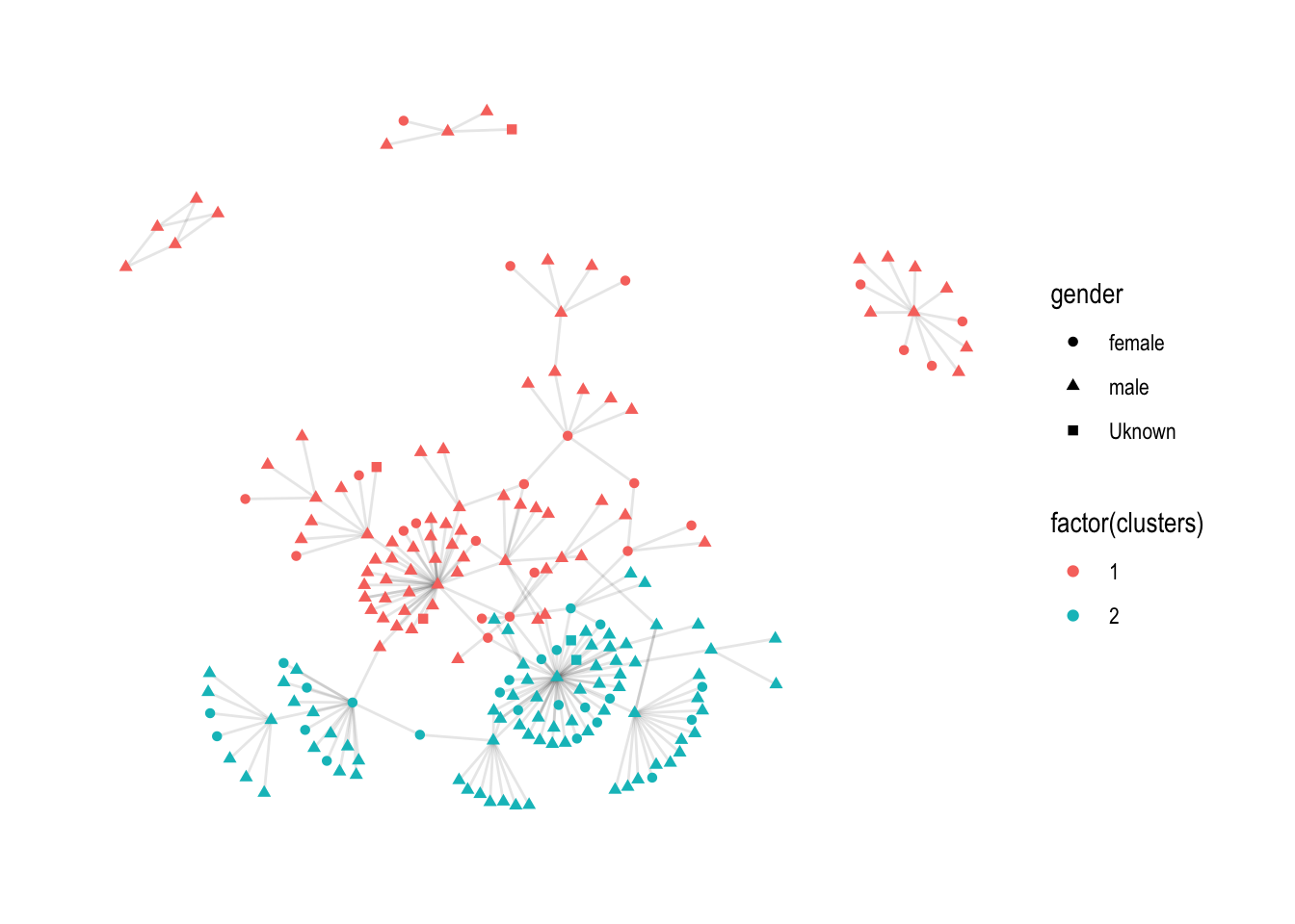
9.2 Christina Prell
# adjacency matrix
prell_adj <- read_csv("https://stulp.gmw.rug.nl/patio/full_100_2SDstrong_asymetric.csv") %>%
  column_to_rownames(var = "...1") # turn column into rownames

prell_nodes <- read.table("https://stulp.gmw.rug.nl/patio//Attrib_image.txt", header = TRUE, sep = "\t") %>%
  rename(organisation = "X")

# Combine adjacancy matrix and node attributes
prell_nw <- as_tbl_graph(prell_adj) %>%
  activate(nodes) %>%
  left_join(prell_nodes, by = c("name" = "organisation"))

prell_nw
## # A tbl_graph: 100 nodes and 881 edges
## #
## # An undirected multigraph with 51 components
## #
## # Node Data: 100 × 7 (active)
## name Mode_n ORG_TYPE Vag_ord indeg_both OutDeg_org Indeg_org
## <chr> <int> <int> <int> <int> <int> <int>
## 1 54events.nl 1 2 2 1 1 1
## 2 allesoverwindenergie.… 1 2 7 1 0 1
## 3 amnesty.org 1 1 6 0 0 0
## 4 anteagroup.nl 1 2 5 0 0 0
## 5 apple.com 1 2 3 0 0 0
## 6 beccuijk.nl 1 2 1 1 0 1
## # … with 94 more rows
## #
## # Edge Data: 881 × 3
## from to weight
## <int> <int> <dbl>
## 1 1 1 1
## 2 4 4 5
## 3 4 8 4
## # … with 878 more rowsNot extremely useful…
# Create bipartite
prell_nw <- prell_nw %>%
  activate(nodes) %>%
  mutate(is_0_type = ORG_TYPE == 0,
         lvl = ORG_TYPE)


ggraph(prell_nw, layout = "fr") +
  geom_edge_link() +
  geom_node_point(aes(colour = factor(ORG_TYPE))) +
  theme_graph()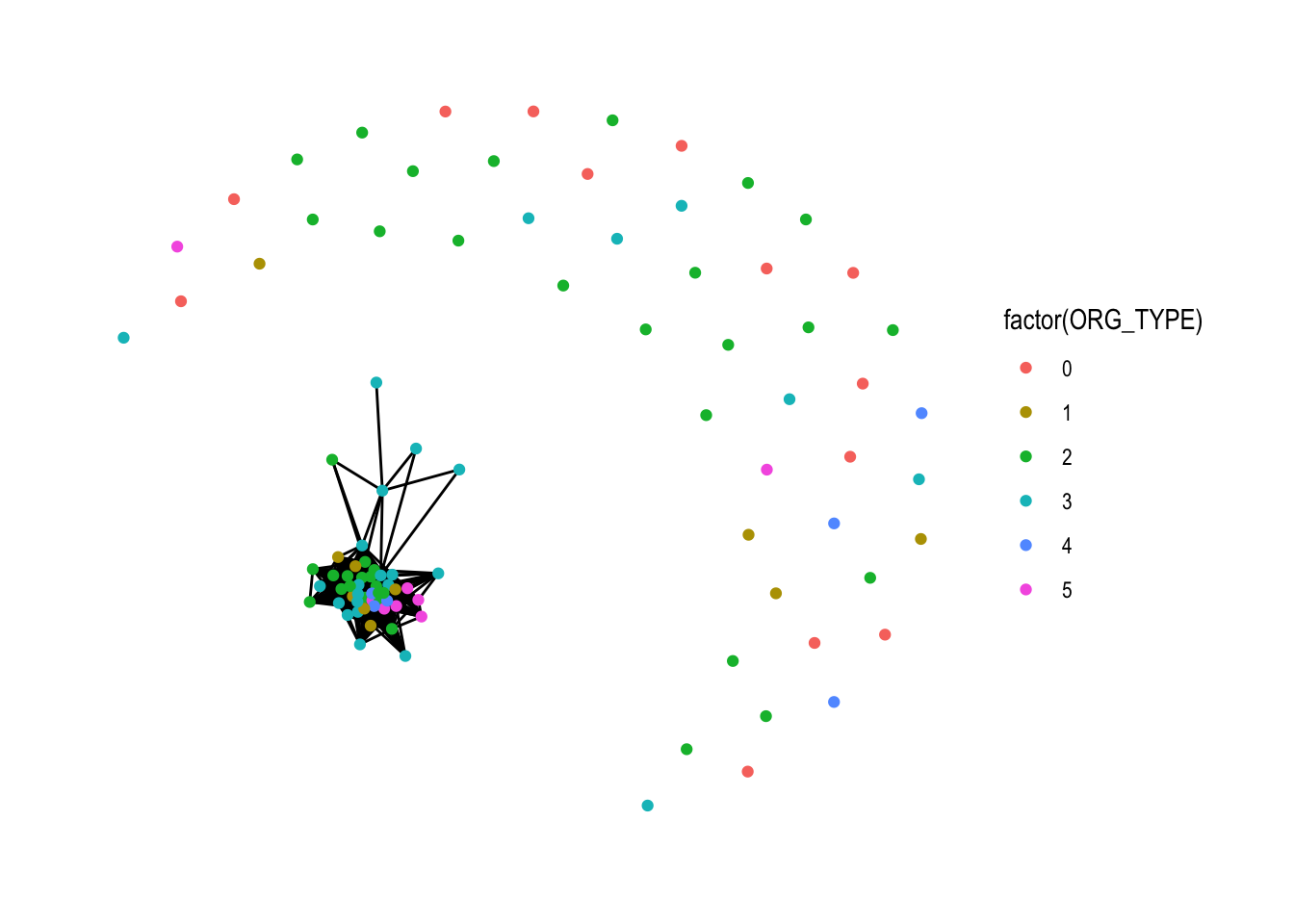
Christina: you’re question was not too easy, here are three potential answers to your question, we can see if we can make it work:
9.3 Annie Kok
(data not available)
library(readxl)

edges_kok <- read_csv("data/afterrobberyedgelist.csv") %>%
  rename(from = "sender",
         to = "receiver") %>%
  mutate(location_num = as.numeric(factor(Location)))

nw_kok <- as_tbl_graph(edges_kok)

nw_kok
## # A tbl_graph: 142 nodes and 323 edges
## #
## # A directed multigraph with 5 components
## #
## # Node Data: 142 × 1 (active)
## name
## <chr>
## 1 Acc_4
## 2 Acc_17
## 3 Unk_8
## 4 Acc_16
## 5 Unk_65
## 6 Unk_97
## # … with 136 more rows
## #
## # Edge Data: 323 × 7
## from to DateTime Location event datetime location_num
## <int> <int> <dbl> <chr> <chr> <chr> <dbl>
## 1 1 82 1159780008 01-RB_Lighthouse-0 after_9 2006/10/02 09:… 2
## 2 1 82 1159812248 01-RB_Lighthouse-0 after_9 2006/10/02 18:… 2
## 3 2 83 1159813735 01-RB_Lighthouse-0 after_9 2006/10/02 18:… 2
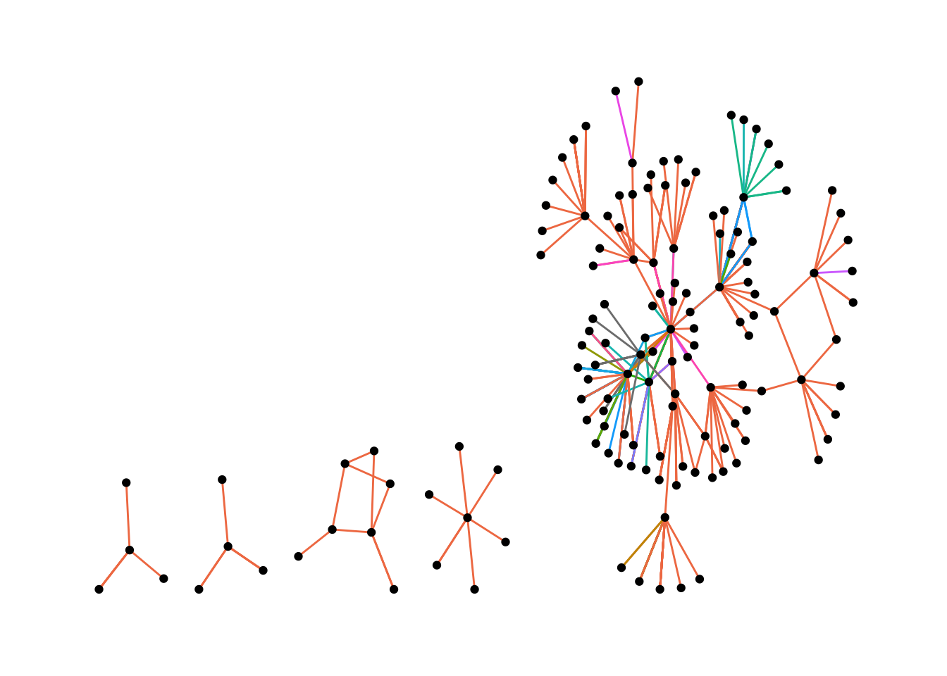
## # … with 320 more rowsggraph(nw_kok, layout = "stress") +
geom_edge_link(aes(colour = factor(location_num))) +
geom_node_point() +
theme_graph() +
theme(
legend.position = "none"
)