Chapter 4 networks are special
A visualization of a network is mostly not overly complicated–typically some circles on an xy-plane with some lines between those circles. Network data, though, is rather curious. This is because a network is typically described by two different bodies of information:
Information on the nodes/vertices/leafs. An easy example is a dataset with the names of individuals and some characteristics of these individuals (e.g., age, sex)
Information on the edges/links/ties. This could be the existence of a tie (A and B know one another), the existence of a directional tie (A considers B a friend), or the strength of that tie (A is “very close” to B). To complicate things, different network data structure/packages favour different kinds of ways to store information on edges. There is for instance the “edge list”, or the “adjacency matrix”. We’ll see examples of each. A network is hardly a network without information on ties, whereas attributes on nodes (except for their “identity”) are optional.
4.1 Visualizing from an edge list
4.1.1 The simplest case
Let’s create an edgelist. We’ll create a dataset called df_edges [this name is arbitrary].
df_edges <- data.frame(
  from = c("Gert","Gert","Gert","Gert","Gert","Ben","Anne"),
  to = c("Anne","Ben","Winy","Vera","Laura","Winy","Vera")
)
If you run this code, you’ll see something appear in your “global environment” [top right corner]. There is an object called df_edges, which is a dataset. Let’s turn it into a network object via the package tidygraph.
# install.packages("tidygraph")
library(tidygraph)

# Create network object from dataframe with edges
nw_obj <- as_tbl_graph(df_edges)

nw_obj
## # A tbl_graph: 6 nodes and 7 edges
## #
## # A directed acyclic simple graph with 1 component
## #
## # Node Data: 6 × 1 (active)
## name
## <chr>
## 1 Gert
## 2 Ben
## 3 Anne
## 4 Winy
## 5 Vera
## 6 Laura
## #
## # Edge Data: 7 × 2
## from to
## <int> <int>
## 1 1 3
## 2 1 2
## 3 1 4
## # … with 4 more rowsThe creation of the network object was a success. We see that the nw_obj (of class tbl_graph) consists of Node Data and Edge Data. So it has created two datasets from our one dataset. Let’s explore both. Because the nw_obj consists of two datasets, we need a way to “tell” the object which dataset we’re interested in if we want to see/change it. We can do this with activate and then specify nodes or edges.
# The `%>%` is called "the pipe" and you can read it as "and then do" or
# "send this thing on the left hand side to the function on the right hand side"
nw_obj %>% activate(nodes)
## # A tbl_graph: 6 nodes and 7 edges
## #
## # A directed acyclic simple graph with 1 component
## #
## # Node Data: 6 × 1 (active)
## name
## <chr>
## 1 Gert
## 2 Ben
## 3 Anne
## 4 Winy
## 5 Vera
## 6 Laura
## #
## # Edge Data: 7 × 2
## from to
## <int> <int>
## 1 1 3
## 2 1 2
## 3 1 4
## # … with 4 more rowsnw_obj %>% activate(edges)## # A tbl_graph: 6 nodes and 7 edges
## #
## # A directed acyclic simple graph with 1 component
## #
## # Edge Data: 7 × 2 (active)
## from to
## <int> <int>
## 1 1 3
## 2 1 2
## 3 1 4
## 4 1 5
## 5 1 6
## 6 2 4
## # … with 1 more row
## #
## # Node Data: 6 × 1
## name
## <chr>
## 1 Gert
## 2 Ben
## 3 Anne
## # … with 3 more rowsThe network object exists, let’s try and visualize via the tidygraph package. The main function to use is ggraph, where the network object is the first “argument”.
# install.packages("ggraph")
library(ggraph)

ggraph(nw_obj)
SUCCES! Sort of. Something happened. Apparently with the sugiyama layout, but we see little evidence of a layout. That’s because we haven’t drawn any edges/ties. We have only defined an empty canvas to draw on!
ggraph(nw_obj) +
  geom_edge_link()
## Using `sugiyama` as default layout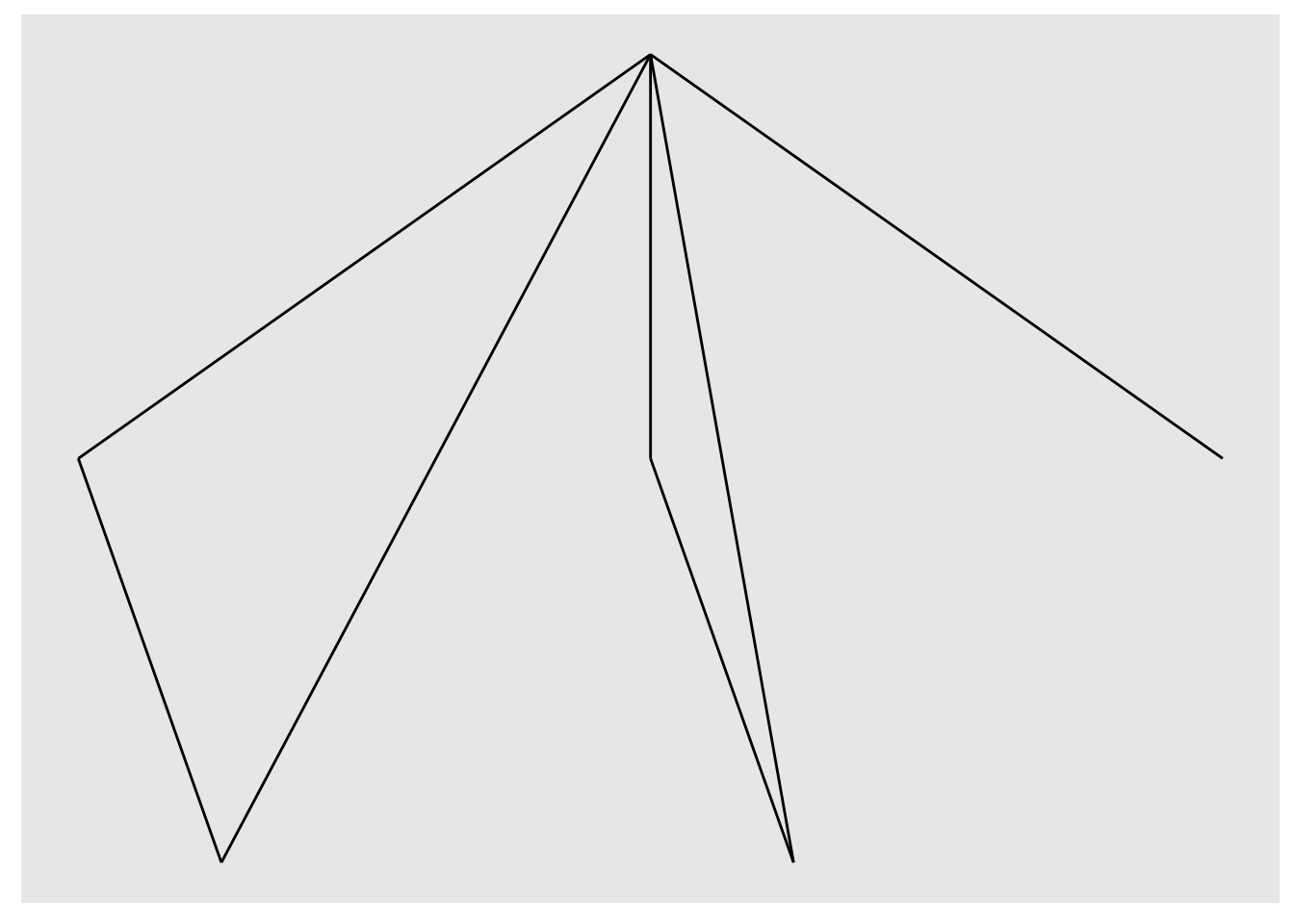
Looks more like a network! Let’s draw some nodes.
ggraph(nw_obj) +
  geom_edge_link() +
  geom_node_point()
## Using `sugiyama` as default layout
Let’s remove that grey background which is part of the theme, by including a theme called theme_graph.
ggraph(nw_obj) +
  geom_edge_link() +
  geom_node_point() +
  theme_graph()
## Using `sugiyama` as default layout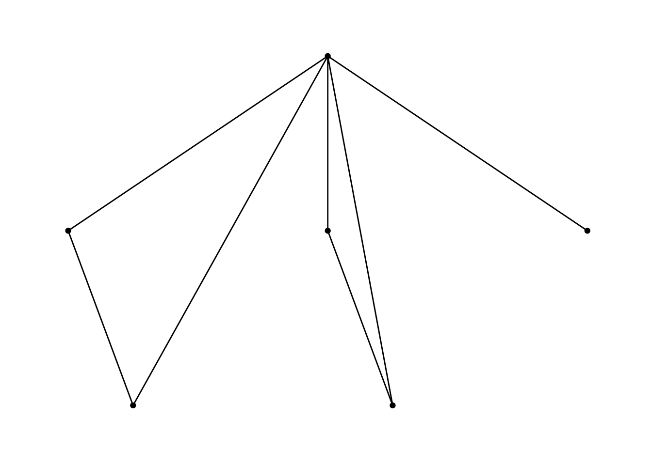
4.2 A slightly more difficult edge list
Let’s have data from a slightly more complicated edge list. Where we also have a variable on tie strength.
df_edges2 <- data.frame(
  closeness = c("very close", "close", "close", "close",
                "somewhat close", "very close", "very close"),
  person1 = c("Gert","Gert","Gert","Gert","Gert","Ben","Anne"),
  person2 = c("Anne","Ben","Winy","Vera","Laura","Winy","Vera")
)
# Create network object from dataframe with edges
nw_obj2 <- as_tbl_graph(df_edges2)
nw_obj2## # A tbl_graph: 6 nodes and 7 edges
## #
## # A directed acyclic multigraph with 1 component
## #
## # Node Data: 6 × 1 (active)
## name
## <chr>
## 1 very close
## 2 close
## 3 somewhat close
## 4 Gert
## 5 Ben
## 6 Anne
## #
## # Edge Data: 7 × 3
## from to person2
## <int> <int> <chr>
## 1 1 4 Anne
## 2 2 4 Ben
## 3 2 4 Winy
## # … with 4 more rowsThat’s not quite right.
To learn what went wrong, we’d have to dive into the helpfunction of as_tbl_graph:
?as_tbl_graphThe relevant bit is under edges:
The terminal nodes of each edge must either be encoded in a to and from column, or in the two first columns, as integers. These integers refer to nodes index.
So we can fix this in two ways.
- By having a column named
toandfrom. Let’s try and rename the columns
df_edges2a <- df_edges2 %>%
  rename(
    from = "person1",
    to = "person2"
  )
df_edges2a
## closeness from to
## 1 very close Gert Anne
## 2 close Gert Ben
## 3 close Gert Winy
## 4 close Gert Vera
## 5 somewhat close Gert Laura
## 6 very close Ben Winy
## 7 very close Anne Veranw_obj2a <- as_tbl_graph(df_edges2a)
nw_obj2a## # A tbl_graph: 6 nodes and 7 edges
## #
## # A directed acyclic simple graph with 1 component
## #
## # Node Data: 6 × 1 (active)
## name
## <chr>
## 1 Gert
## 2 Ben
## 3 Anne
## 4 Winy
## 5 Vera
## 6 Laura
## #
## # Edge Data: 7 × 3
## from to closeness
## <int> <int> <chr>
## 1 1 3 very close
## 2 1 2 close
## 3 1 4 close
## # … with 4 more rowsSuccess. The other method involves rearranging the columns, where the first two columns will be used.
df_edges2b <- df_edges2 %>%
  select(person1, person2, closeness) # rearrange order variables

df_edges2b
## person1 person2 closeness
## 1 Gert Anne very close
## 2 Gert Ben close
## 3 Gert Winy close
## 4 Gert Vera close
## 5 Gert Laura somewhat close
## 6 Ben Winy very close
## 7 Anne Vera very closenw_obj2b <- as_tbl_graph(df_edges2b)
nw_obj2b## # A tbl_graph: 6 nodes and 7 edges
## #
## # A directed acyclic simple graph with 1 component
## #
## # Node Data: 6 × 1 (active)
## name
## <chr>
## 1 Gert
## 2 Ben
## 3 Anne
## 4 Winy
## 5 Vera
## 6 Laura
## #
## # Edge Data: 7 × 3
## from to closeness
## <int> <int> <chr>
## 1 1 3 very close
## 2 1 2 close
## 3 1 4 close
## # … with 4 more rowsYet another success.
Let’s see if we can use that information from the closeness variable.
ggraph(nw_obj2a) +
  geom_edge_link(aes(colour = closeness)) +
  geom_node_point() +
  theme_graph()
## Using `sugiyama` as default layout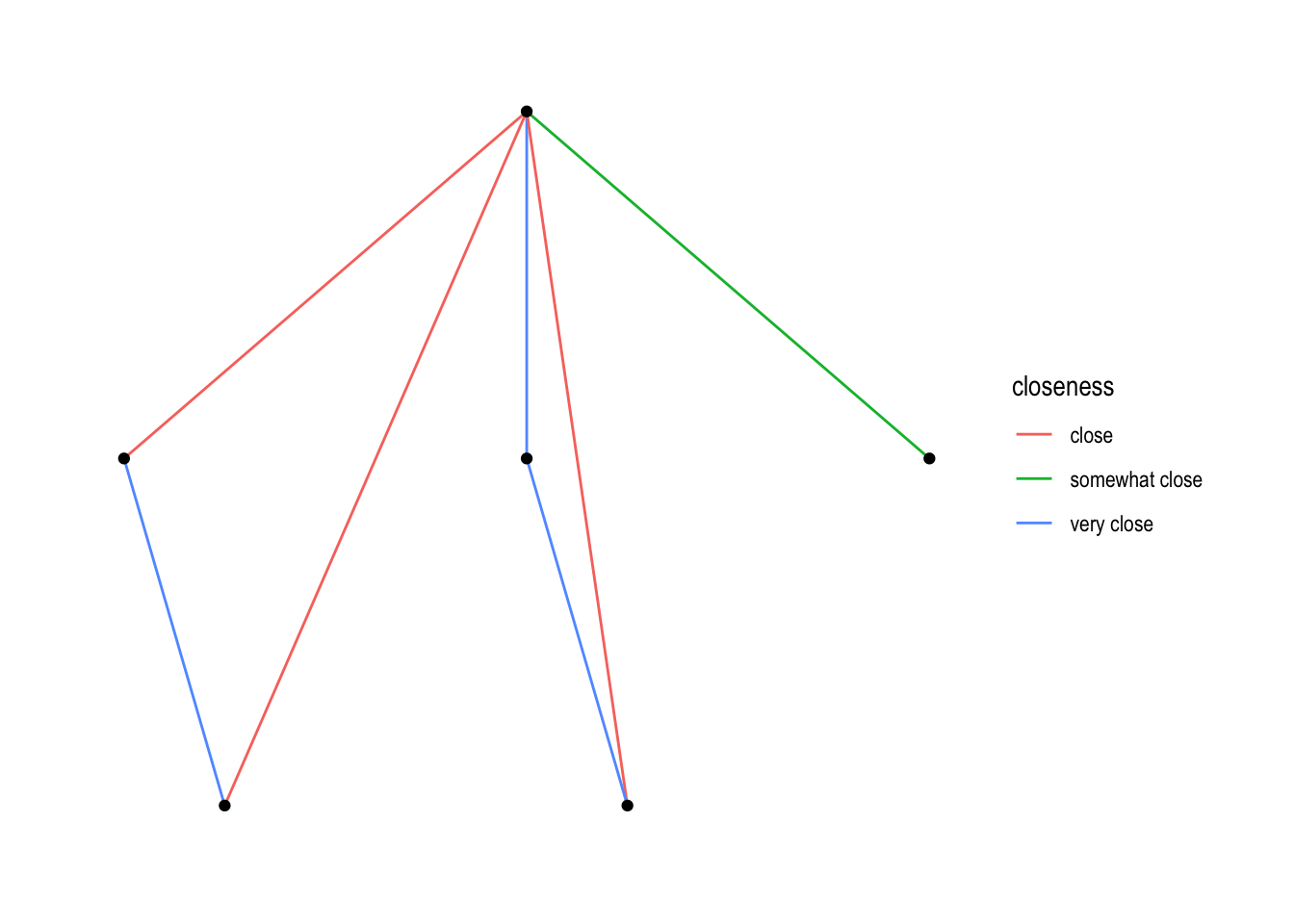
In the above code aes refers to “aesthetics”. Within those brackets you can “map” variables to “aesthetics”. Here we “map” the variable closeness to colour. We could have also done edge_width (or edge_alpha, or edge_linetype or …, see section “Edges”):
ggraph(nw_obj2a) +
  geom_edge_link(aes(edge_width = closeness)) +
  geom_node_point() +
  theme_graph()
## Using `sugiyama` as default layout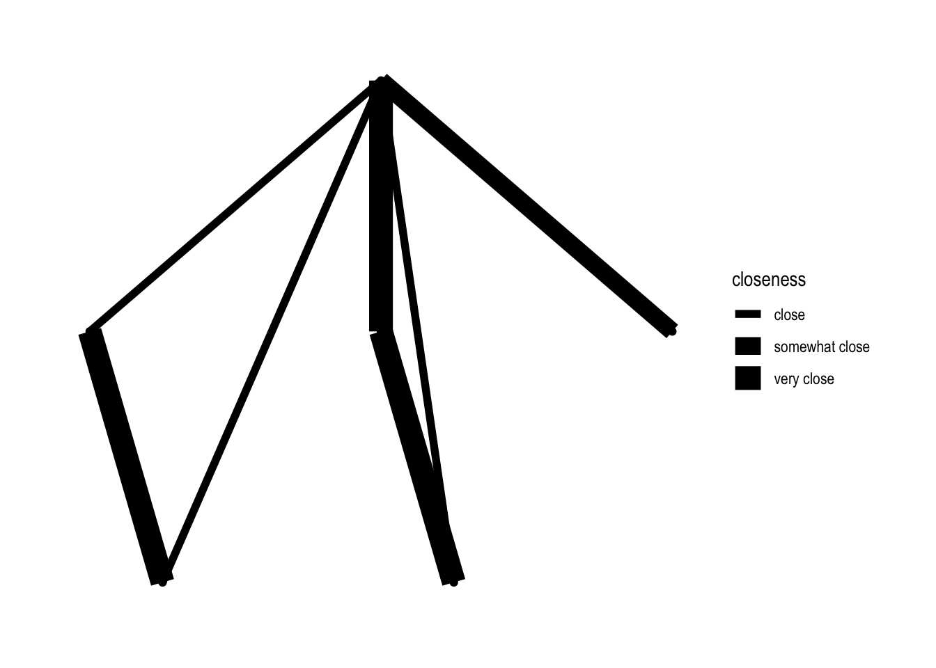
Well, that’s no improvement!
4.3 An adjacancy matrix
It works more or less similar when providing adjacency matrices. Let’s create an undirected one:
adj1 <- matrix(c(1, 0, 1,
                 0, 1, 1,
                 1, 1, 1), nrow = 3, ncol = 3)
nw_obj3 <- as_tbl_graph(adj1, directed = FALSE)
nw_obj3## # A tbl_graph: 3 nodes and 5 edges
## #
## # An undirected multigraph with 1 component
## #
## # Node Data: 3 × 0 (active)
## #
## # Edge Data: 5 × 3
## from to weight
## <int> <int> <dbl>
## 1 1 1 1
## 2 1 3 1
## 3 2 2 1
## # … with 2 more rowsggraph(nw_obj3) +
geom_edge_link() +
geom_node_point() +
theme_graph()## Using `stress` as default layout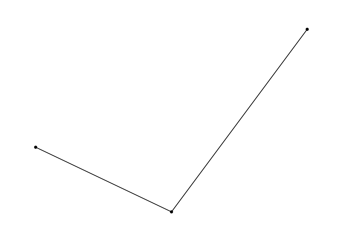
Let’s create a directed adjacency matrix, with tie strength information.
adj2 <- matrix(c(1, 2, 3,
                 0, 1, 4,
                 0, 4, 1), nrow = 3, ncol = 3)
nw_obj4 <- as_tbl_graph(adj2)
nw_obj4## # A tbl_graph: 3 nodes and 7 edges
## #
## # A directed multigraph with 1 component
## #
## # Node Data: 3 × 0 (active)
## #
## # Edge Data: 7 × 3
## from to weight
## <int> <int> <dbl>
## 1 1 1 1
## 2 2 1 2
## 3 2 2 1
## # … with 4 more rowsggraph(nw_obj4) +
geom_edge_link() +
geom_node_point() +
theme_graph()## Using `stress` as default layout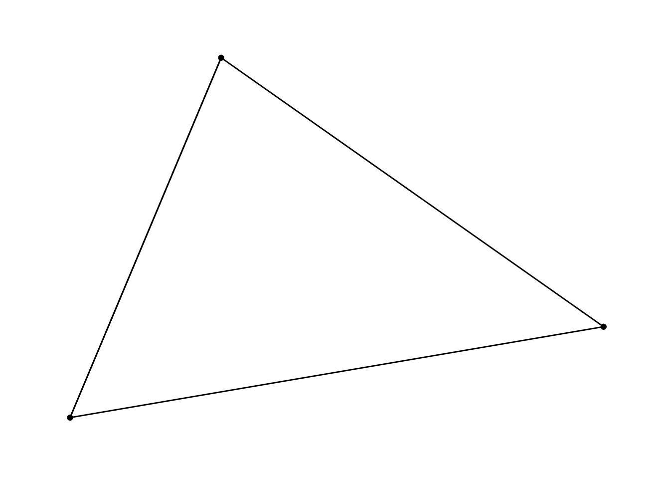
Let’s do something more radical:
ggraph(nw_obj4) +
  geom_edge_arc(
    aes(colour = factor(weight)),
    arrow = arrow(length = unit(4, 'mm')),
    end_cap = circle(3, 'mm')
  ) +
  geom_node_point() +
  theme_graph()
## Using `stress` as default layout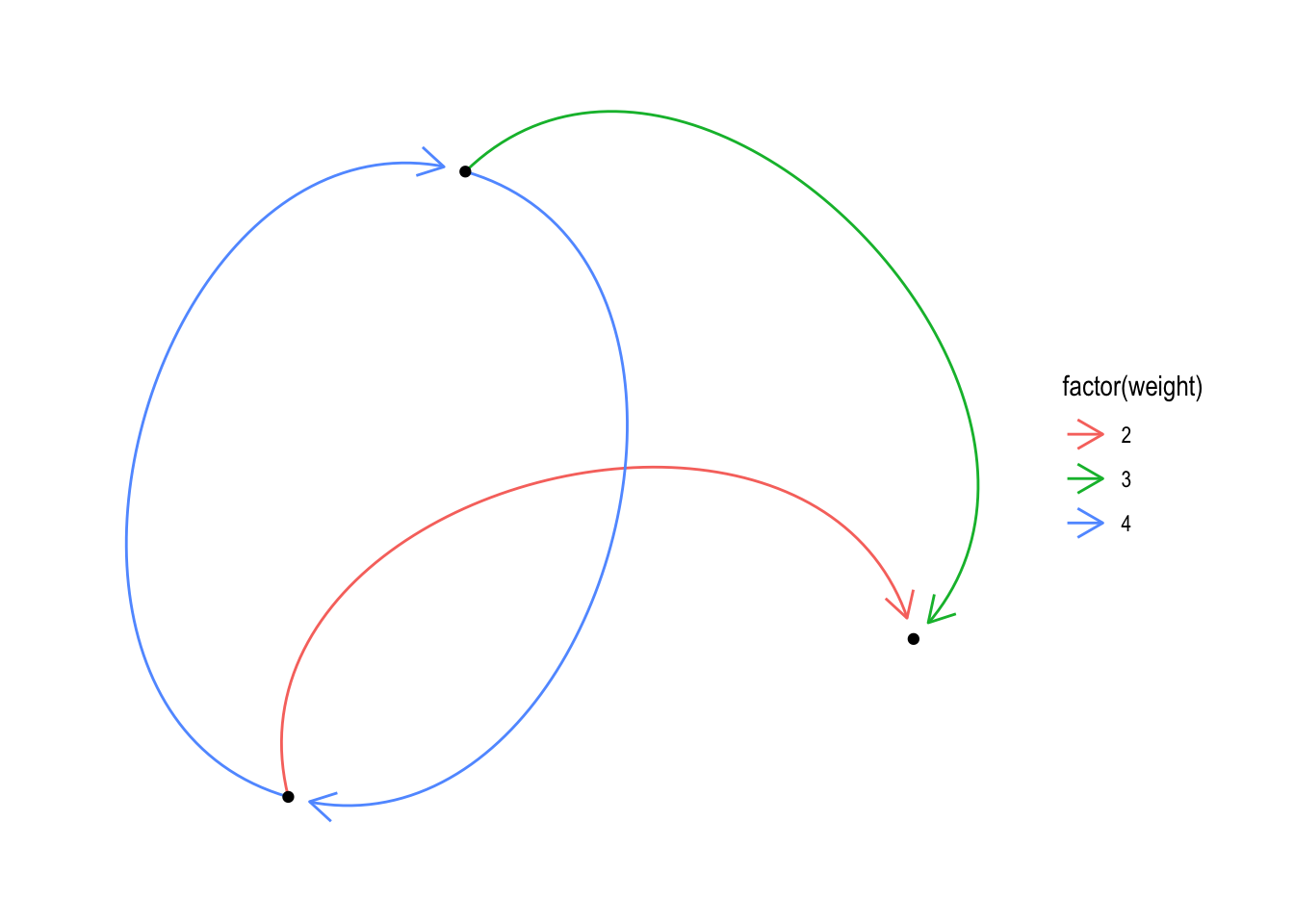
4.4 Combining data on note attributes and an edge list
df_edges <- data.frame(
  from = c("Gert","Gert","Gert","Gert","Gert","Ben","Anne"),
  to = c("Anne","Ben","Winy","Vera","Laura","Winy","Vera"),
  closeness = c("very close", "close", "close", "close", "somewhat close",
                "very close", "very close")
)

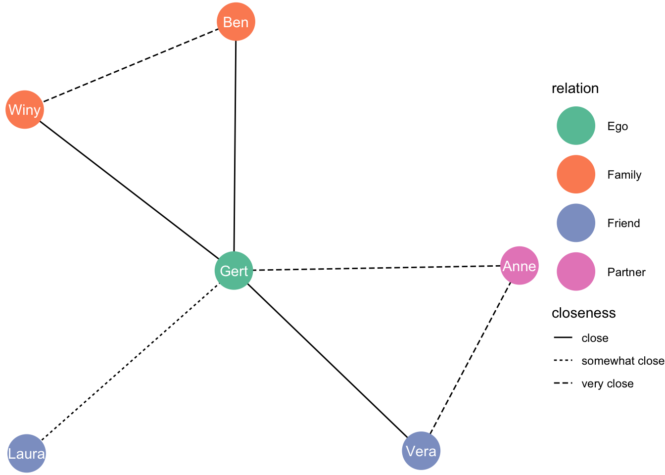
df_nodes <- data.frame(
  name = c("Gert", "Anne", "Ben", "Winy", "Vera", "Laura"),
  relation = c("Ego", "Partner", "Family", "Family", "Friend", "Friend")
)

df_network <- tbl_graph(nodes = df_nodes, edges = df_edges, directed = FALSE)

df_network
## # A tbl_graph: 6 nodes and 7 edges
## #
## # An undirected simple graph with 1 component
## #
## # Node Data: 6 × 2 (active)
## name relation
## <chr> <chr>
## 1 Gert Ego
## 2 Anne Partner
## 3 Ben Family
## 4 Winy Family
## 5 Vera Friend
## 6 Laura Friend
## #
## # Edge Data: 7 × 3
## from to closeness
## <int> <int> <chr>
## 1 1 2 very close
## 2 1 3 close
## 3 1 4 close
## # … with 4 more rowsThe simplest one possible:
ggraph(df_network, layout = "kk") +
  geom_node_point() +
  geom_edge_link() +
  theme_graph()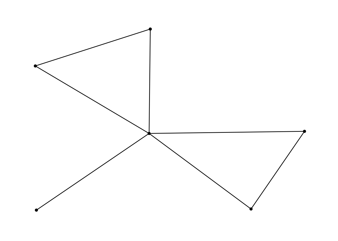
ggraph(df_network, layout = "kk") +
  geom_edge_link(aes(linetype = closeness)) +
  geom_node_point(aes(colour = relation), size = 13) +
  geom_node_text(aes(label = name), colour = "white") +
  theme_void() +
  scale_color_brewer(palette = "Set2")