Chapter 8 network data visualization 2.0

We’ve seen how to change the basic elements of any network graph. Now, let’s level it up. Let’s calculate various network metrics and incorporate them into our network visualizations.

Let’s go back to those striped animals again. Data from this wonderful website.:

zebra_graphml <- read.graph("https://raw.githubusercontent.com/bansallab/asnr/master/Networks/Mammalia/zebra_groupmembership_weighted/zebra_sundaresan_interaction_attribute.graphml", format = "graphml")

zebra <- as_tbl_graph(zebra_graphml)

ggraph(zebra, layout = "kk") +
  geom_edge_link(colour = "grey", alpha = 0.5) +
  geom_node_point(colour = "orange", size = 7) +
  geom_node_text(aes(label = id), colour = "white") +
  theme_graph()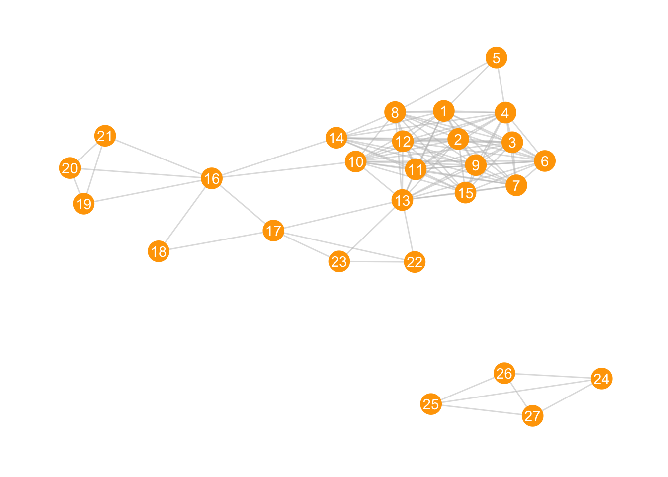 

8.1 Components

We see two clear components (groups of nodes with ties between them, but not between members of other groups). How can we give those two components different colours?

We’ll first have to calculate the number of components, and decide which nodes belong to which component. Luckily, the package igraph has a function called components. The output of that function is a list of three things. We’re interested in the membership.

zebra <- zebra %>% 
  activate(nodes) %>% 
  mutate(components = components(.)$membership)

ggraph(zebra, layout = "kk") +
  geom_edge_link(colour = "grey", alpha = 0.5) +
  geom_node_point(aes(colour = factor(components)), size = 7) +
  geom_node_text(aes(label = id), colour = "white") +
  theme_graph() +
  scale_colour_manual(values = c("#CC79A7", "#56B4E9"))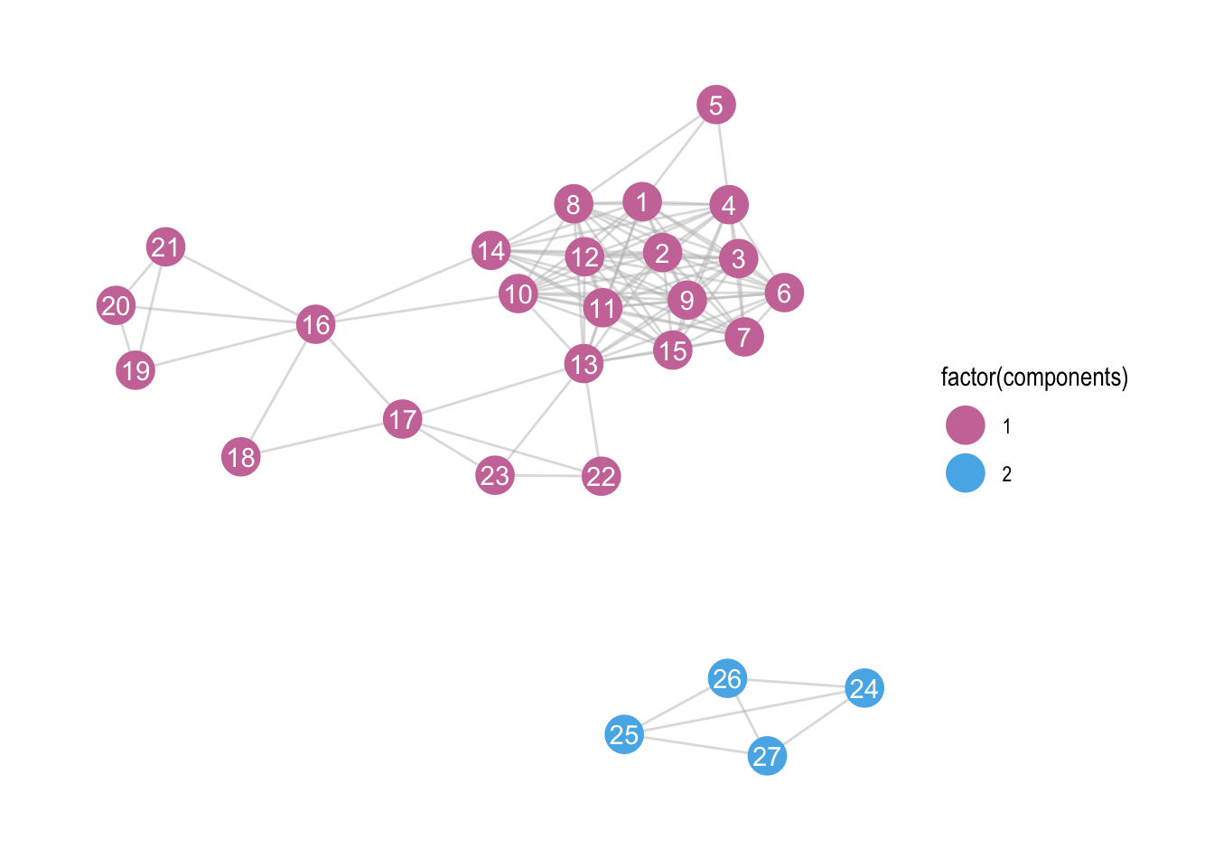 

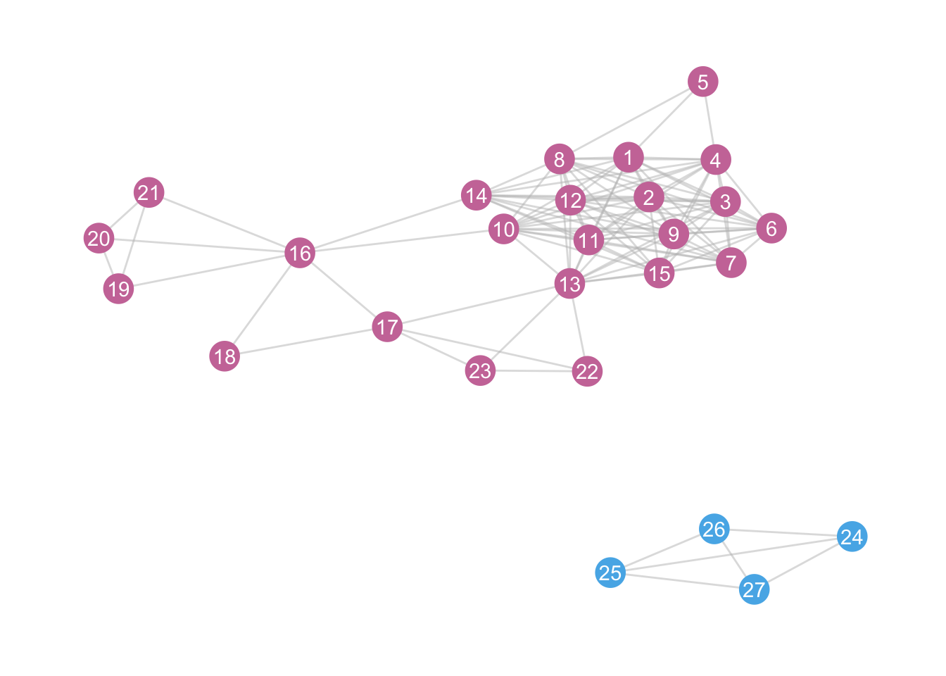
Note that the package tidygraph also has a ‘wrapper’ around all the igraph functions. This does the same (I have also removed the legend):

zebra <- zebra %>% 
  activate(nodes) %>% 
  mutate(components2 = group_components())

ggraph(zebra, layout = "kk") +
  geom_edge_link(colour = "grey", alpha = 0.5) +
  geom_node_point(aes(colour = factor(components2)), size = 7) +
  geom_node_text(aes(label = id), colour = "white") +
  theme_graph() +
  scale_colour_manual(values = c("#CC79A7", "#56B4E9")) +
  theme(
    legend.position = "none"
  )

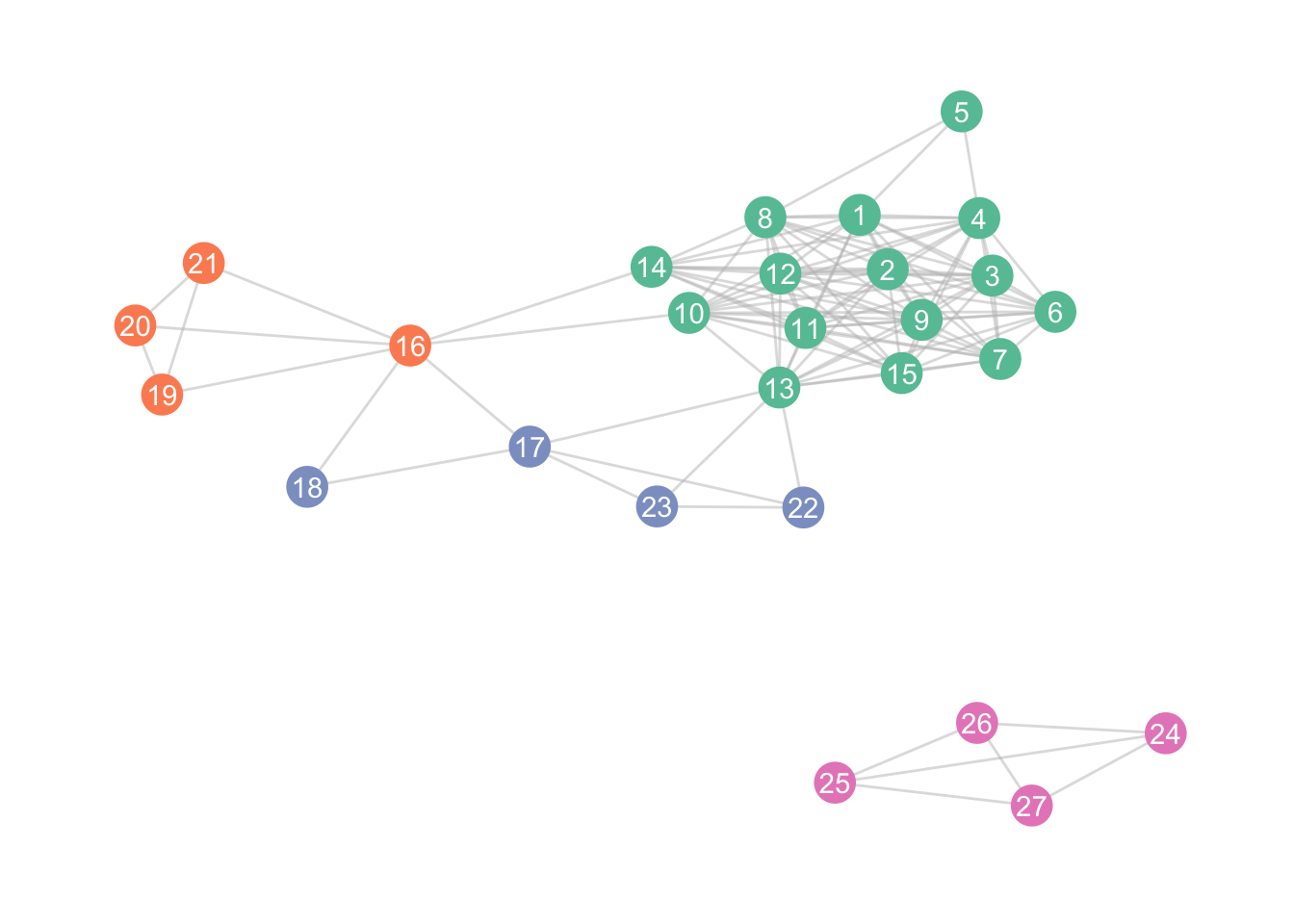
8.2 Communities

We can also define clusters in different ways, for instance, by defining them by “minimiz[ing] the expected description length of a random walker trajectory”

zebra <- zebra %>% 
  activate(nodes) %>% 
  mutate(clusters = group_infomap()) 
# mutate(clusters = membership(cluster_infomap(.))) would also work! 

ggraph(zebra, layout = "kk") +
  geom_edge_link(colour = "grey", alpha = 0.5) +
  geom_node_point(aes(colour = factor(clusters)), size = 7) +
  geom_node_text(aes(label = id), colour = "white") +
  theme_graph() +
  scale_colour_brewer(palette = "Set2") +
  theme(
    legend.position = "none"
  )

8.3 Centrality of nodes

Much of network analysis relies on some form of centrality of particular nodes. Let’s see how we can incorporate that information.

zebra <- zebra %>% 
  activate(nodes) %>% 
  mutate(centrality = centrality_betweenness()) 
# mutate(centrality2 = betweenness(.)) is the same

ggraph(zebra, layout = "kk") +
  geom_edge_link(colour = "grey", alpha = 0.5) +
  geom_node_point(aes(colour = centrality), size = 7) +
  geom_node_text(aes(label = id), colour = "white") +
  theme_graph() +
  scale_colour_viridis_c()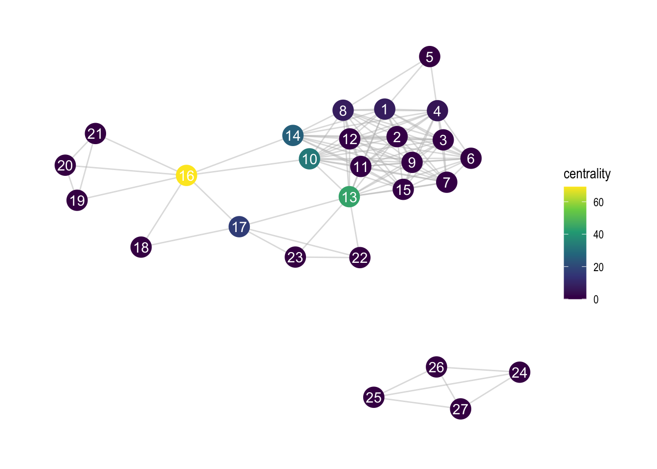 

8.4 Distance from nodes

zebra <- zebra %>% 
  activate(nodes) %>% 
  mutate(is_13 = if_else(id == 13, TRUE, FALSE),
         dist_to_13 = node_distance_to(is_13)) 

ggraph(zebra, layout = "kk") +
  geom_edge_link(colour = "grey", alpha = 0.5) +
  geom_node_point(aes(colour = factor(dist_to_13)), size = 7) +
  geom_node_text(aes(label = id), colour = "white") +
  theme_graph() +
  scale_colour_viridis_d()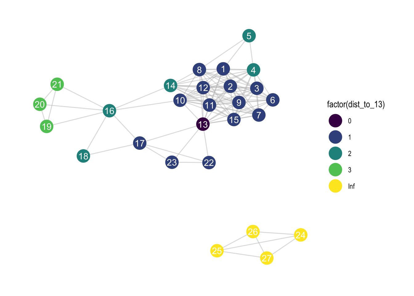 

8.5 A worked example

Let’s do something for dolphins this time! Data from this wonderful website.

dolphins_graphml <- read.graph("https://raw.githubusercontent.com/bansallab/asnr/master/Networks/Mammalia/dolphin_association_weighted/weighted_FORAGE_dolphin_florida.graphml", format = "graphml")

dolphins <- as_tbl_graph(dolphins_graphml)

8.5.1 Descriptives

Let’s get some descriptives first.

How many dolphins are there in the network:

no_nodes <- dolphins %>% 
  activate(nodes) %>% 
  as_tibble() %>% # turns the node characteristics into tibble (dataframe)
  nrow() # count number of rows of node characteristics (= # nodes)

no_nodes

## [1] 190

# alternative way:
# igraph::gorder(dolphins)

How many components are there?

no_comp <- dolphins %>% 
  activate(nodes) %>%
  mutate(components = group_components()) %>% # count # components
  pull(components) %>% # extract only variable named "components"
  max()

no_comp

## [1] 6

# igraph does this more simply
# igraph::components(dolphins)$no

Density of network?

density <- dolphins %>% 
  activate(edges) %>%
  as_tibble() %>% # turns the node characteristics into tibble (dataframe)
  nrow() / ( (190 * 189) / 2  ) # count number of edges / total undirected edges
  
density

## [1] 0.06315789

# igraph does this more simply
# igraph::edge_density(dolphins)
# same as 
# igraph::gsize(dolphins) / ( (190 * 189) / 2  )

How many communities are there, if we base it on “Infomap community finding”, which is defined by “Find community structure that minimizes the expected description length of a random walker trajectory”

# let's keep results, so we can use it later in the visualization
dolphins <- dolphins %>% 
  activate(nodes) %>% 
  mutate(clusters = group_infomap())

no_clusters <- dolphins %>% 
  activate(nodes) %>%
  pull(clusters) %>% # extract only variable named "components"
  max()

no_clusters

## [1] 24

# igraph does this more simply
# length(igraph::cluster_infomap(dolphins))

8.5.2 Let’s visualise

ggraph(dolphins, layout = "fr") +
  geom_edge_link(alpha = 0.2) +
  geom_node_point() +
  theme_graph()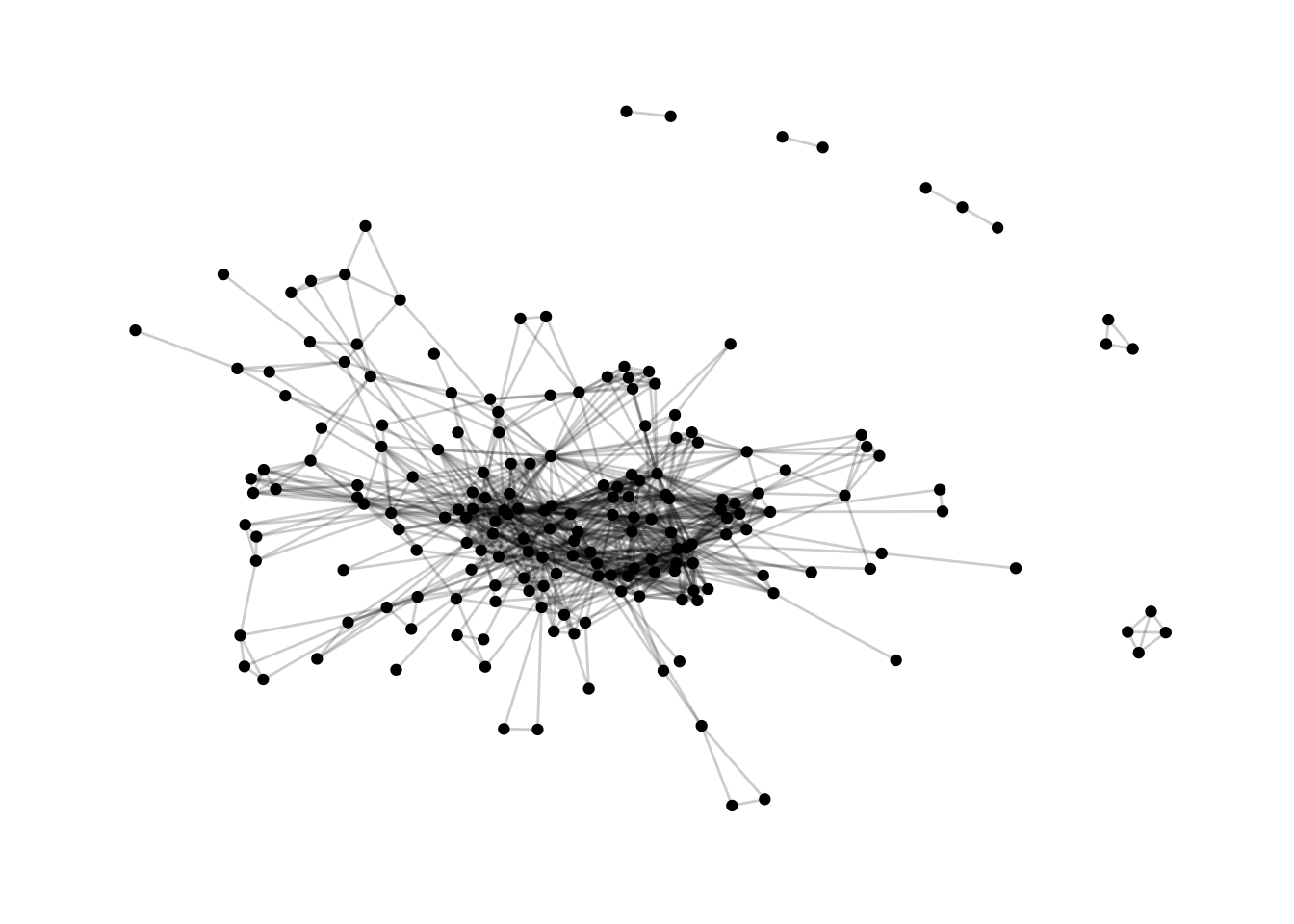

Let’s try and add some information:

set.seed(1)
ggraph(dolphins, layout = "fr") +
  geom_edge_link(alpha = 0.2) +
  geom_node_point() +
  theme_minimal() +
  theme_graph() +
  annotate("text", label = paste0("n: ", no_nodes, " dolphins"), 
           x = 12.5, y = 14, hjust = 1) +
  annotate("text", label = paste0("density: ", round(100 * density), "%"), 
           x = 12.5, y = 12.5, hjust = 1) +
  annotate("text", label = paste0("# clusters: ", no_clusters), 
           x = 12.5, y = 11, hjust = 1)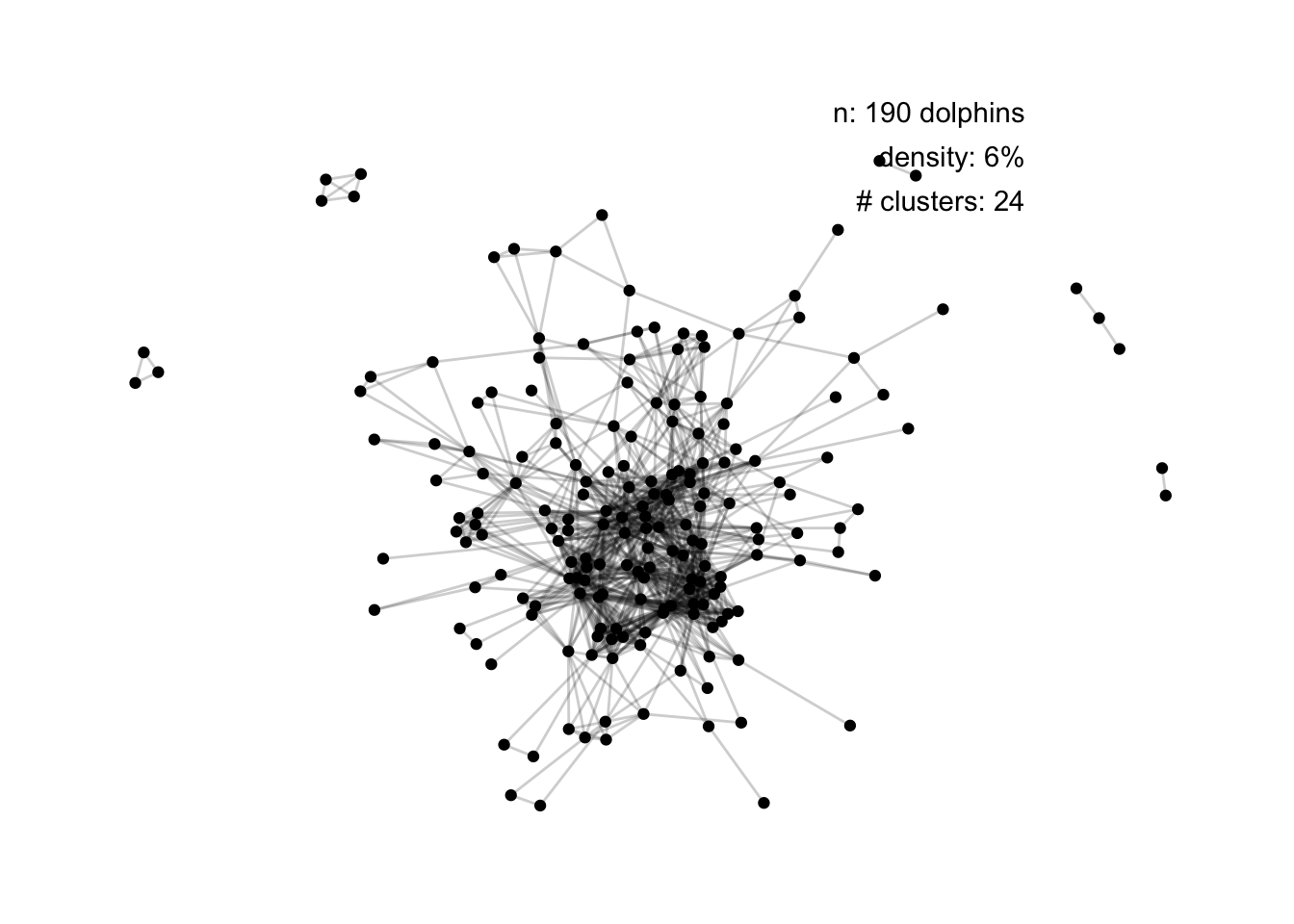 

set.seed(1)
ggraph(dolphins, layout = "fr") +
  geom_edge_link(alpha = 0.2) +
  geom_node_point(aes(colour = factor(clusters))) +
  theme_minimal() + 
  theme_graph() +
  annotate("text", label = paste0("n: ", no_nodes, " dolphins"), 
           x = 12.5, y = 14, hjust = 1) +
  annotate("text", label = paste0("density: ", round(100 * density), "%"), 
           x = 12.5, y = 12.5, hjust = 1) +
  annotate("text", label = paste0("# clusters: ", no_clusters), 
           x = 12.5, y = 11, hjust = 1) +
  scale_colour_viridis_d() + 
  theme(
    legend.position = "none"
  )

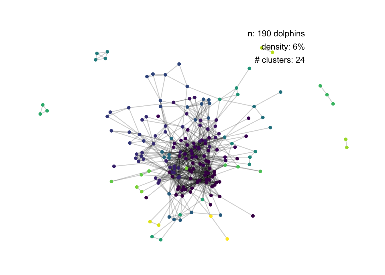
Too many clusters for it to really work.

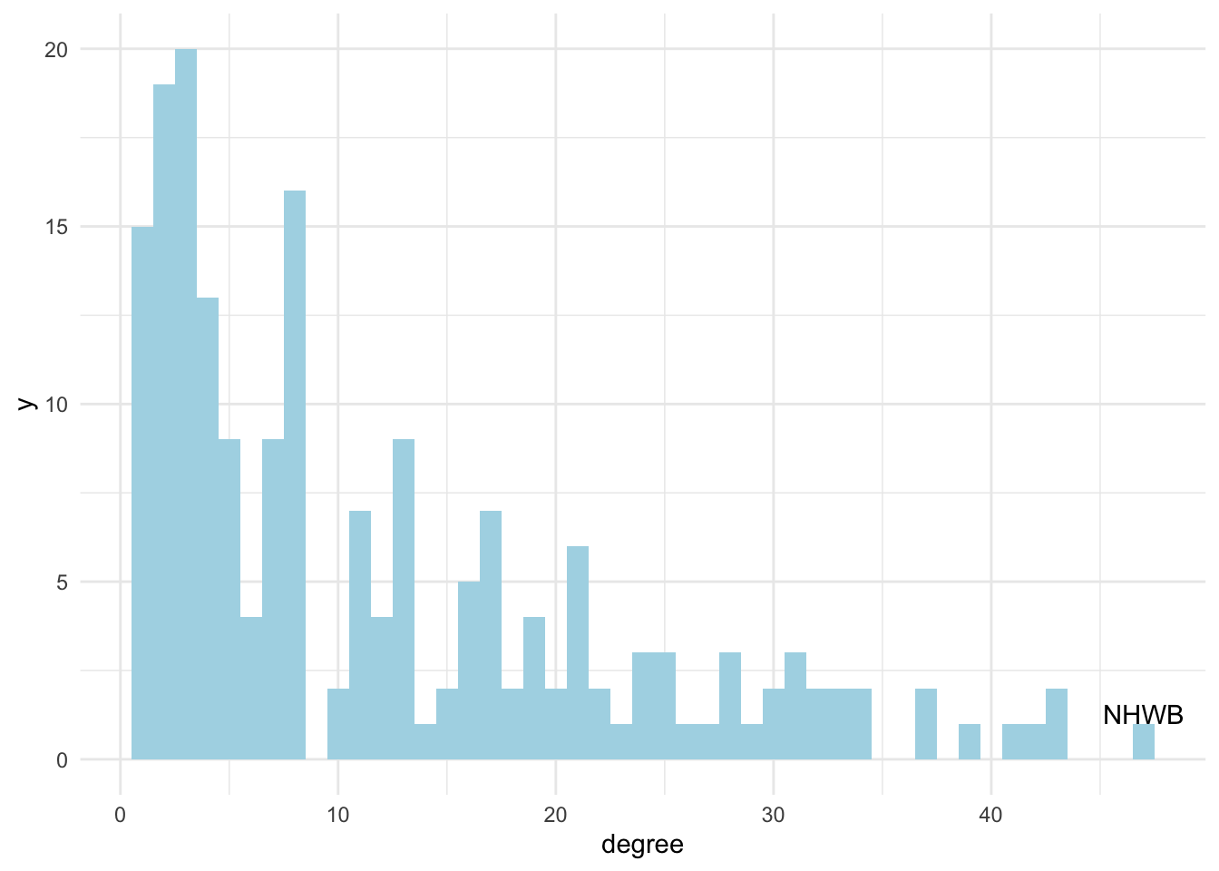
Let’s try one more thing. Let’s say we’re interested in finding out well-connected individuals based on how many ties go into/out of this dolphin (i.e., degree).

dolphins <- dolphins %>% 
  activate(nodes) %>% 
  mutate(degree = degree(.)) # degree is function from igraph

Which dolphin has the maximum degree, and how much is it?

degree_summ <- dolphins %>% 
  activate(nodes) %>% 
  as_tibble() %>% 
  filter(degree == max(degree))

degree_summ

## # A tibble: 1 × 3
##   id    clusters degree
##   <chr>    <int>  <dbl>
## 1 NHWB         1     47

Let’s visualise the variation in degree across the network:

dolphins %>% 
  activate(nodes) %>% 
  as_tibble() %>% 
  ggplot(aes(x = degree)) +
  geom_histogram(binwidth = 1, fill = "lightblue") +
  theme_minimal() +
  annotate("text", x = degree_summ$degree, y = 1, label = degree_summ$id, vjust = 0)