Chapter 6 edges
6.1 Edge attributes
On the basis of data from Lemurs (!) we’ll see which attributes we can vary from edges.

Data from this wonderful website.
lemur_graphml <- read.graph("https://raw.githubusercontent.com/bansallab/asnr/master/Networks/Mammalia/lemur_sexual_weighted/lemur_pereira_sexual_network_1_attribute.graphml", format = "graphml")

lemur <- as_tbl_graph(lemur_graphml)

lemur
## # A tbl_graph: 9 nodes and 7 edges
## #
## # An unrooted forest with 2 trees
## #
## # Node Data: 9 × 3 (active)
## `residence status` SEX id
## <chr> <chr> <chr>
## 1 "immigrant" MALE A
## 2 "resident" FEMALE TR
## 3 "" MALE G
## 4 "resident" FEMALE CN
## 5 "resident" FEMALE LY
## 6 "immigrant" MALE N
## # … with 3 more rows
## #
## # Edge Data: 7 × 3
## from to weight
## <int> <int> <dbl>
## 1 1 2 1
## 2 3 4 1
## 3 3 5 1
## # … with 4 more rowsThe standard graph would look something like this:
ggraph(lemur, layout = "kk") +
  geom_edge_link() +
  geom_node_point(size = 4) +
  theme_graph()
6.1.1 edge colour
An important distinction is that between “setting” and “mapping” variables. Let’s use the colour of edges to see the difference. We could simply ‘set’ the colour of the lines in the following way:
ggraph(lemur, layout = "kk") +
  geom_edge_link(colour = "purple") +
  geom_node_point(size = 4) +
  theme_graph()
A slightly more interesting thing would be to map a variable to the colour of the lines. For example:
ggraph(lemur, layout = "kk") +
  geom_edge_link(aes(colour = factor(weight))) +
  geom_node_point(size = 4) +
  theme_graph()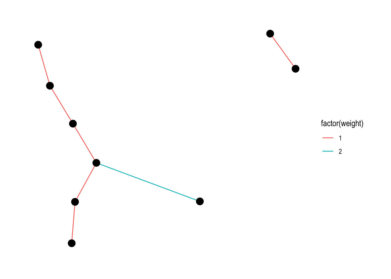
Those colours are not so nice, let’s try to choose our own colours:
ggraph(lemur, layout = "kk") +
  geom_edge_link(aes(colour = factor(weight))) +
  geom_node_point(size = 4) +
  theme_graph() +
  scale_edge_colour_brewer(palette = "Set1")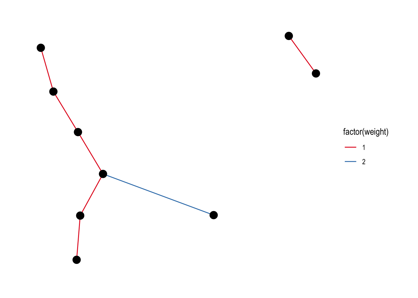
6.1.2 edge width
We can do the same tricks for line width as we did for colour:
Setting the width:
ggraph(lemur, layout = "kk") +
  geom_edge_link(width = 4, colour = "grey") +
  geom_node_point(size = 4) +
  theme_graph()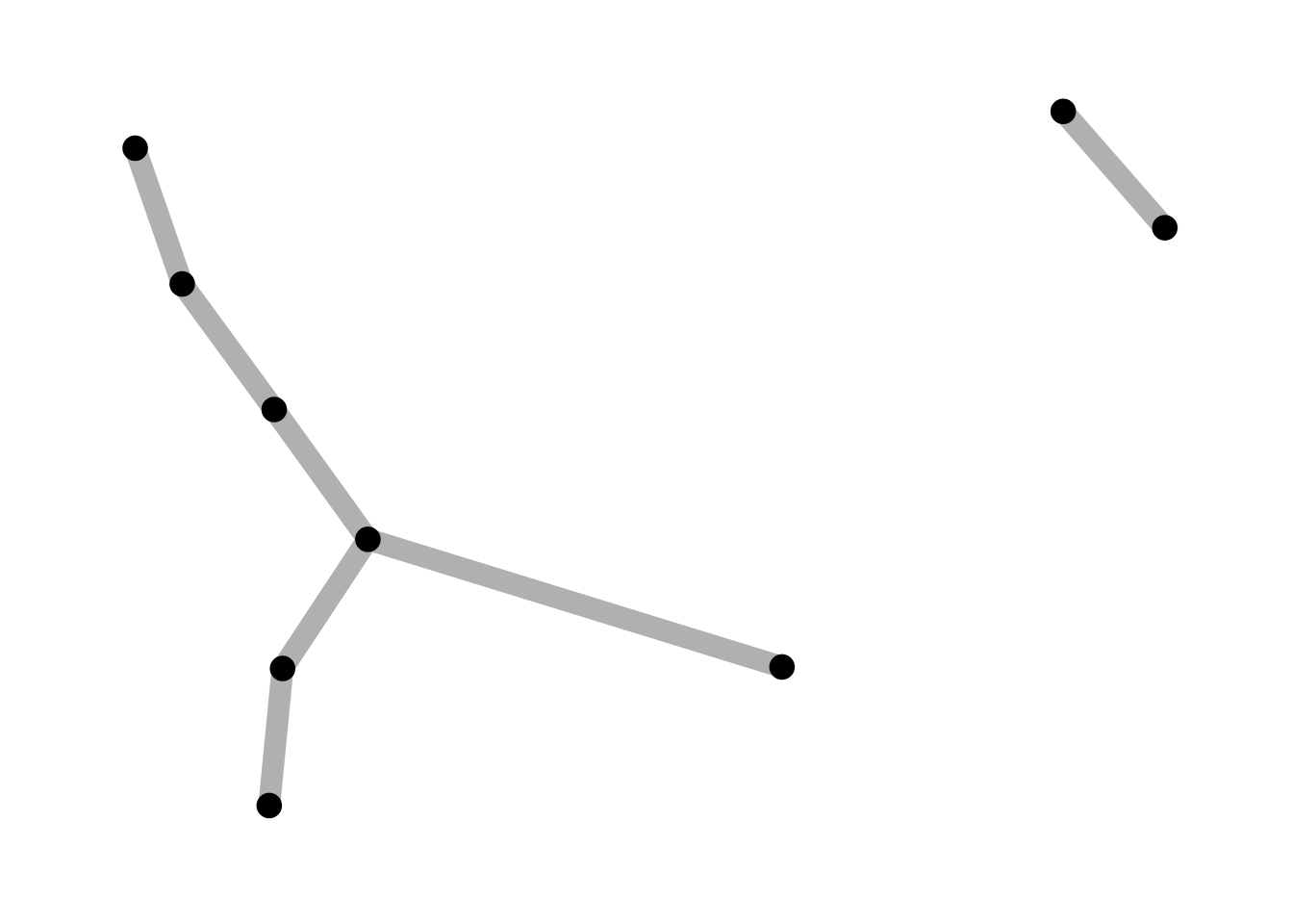
Mapping a variable to width:
ggraph(lemur, layout = "kk") +
  geom_edge_link(aes(width = factor(weight)), colour = "grey") +
  geom_node_point(size = 4) +
  theme_graph()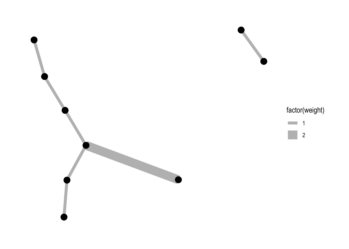
6.1.3 linetype
Setting:
ggraph(lemur, layout = "kk") +
  geom_edge_link(linetype = "dashed") +
  geom_node_point(size = 4) +
  theme_graph()
Mapping:
ggraph(lemur, layout = "kk") +
  geom_edge_link(aes(linetype = factor(weight))) +
  geom_node_point(size = 4) +
  theme_graph()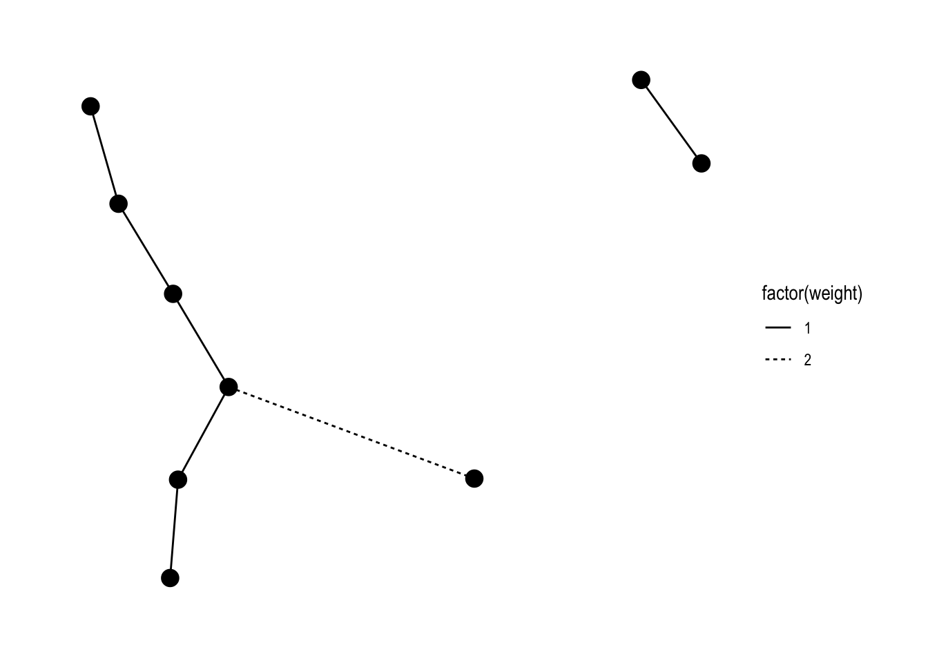
6.1.4 seethroughness
Setting:
ggraph(lemur, layout = "kk") +
  geom_edge_link(alpha = 0.5) +
  geom_node_point(size = 4) +
  theme_graph()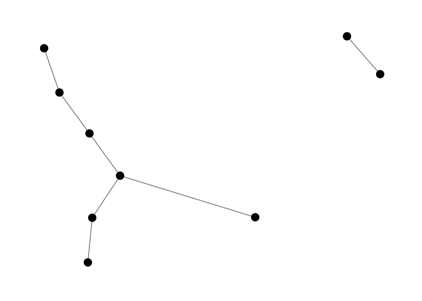
Mapping:
ggraph(lemur, layout = "kk") +
  geom_edge_link(aes(alpha = factor(weight))) +
  geom_node_point(size = 4) +
  theme_graph()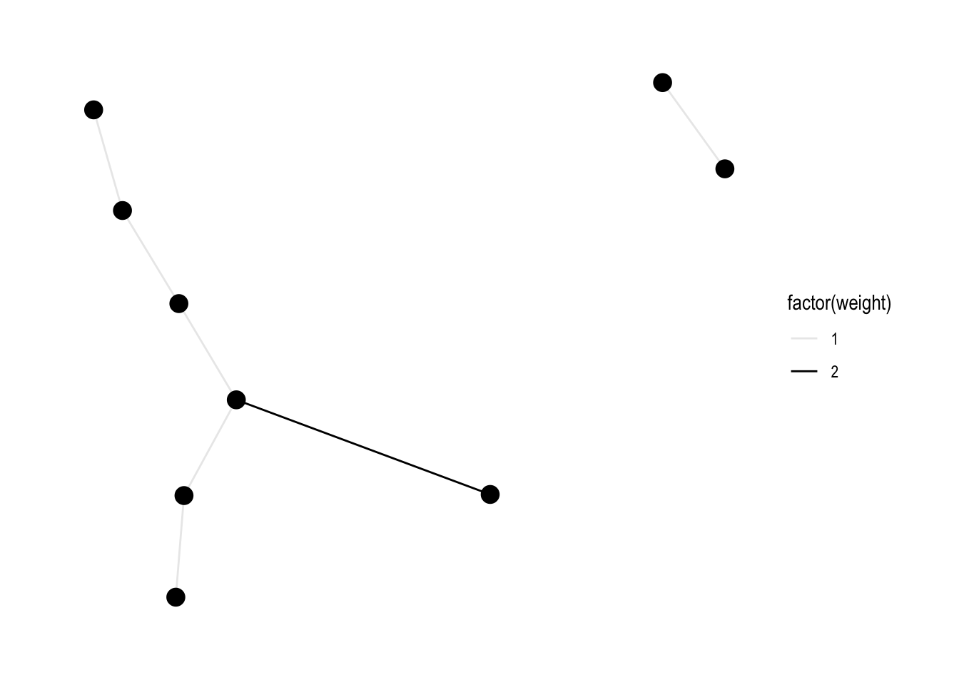
As we’ve seen, alpha is useful when you have many, many edges:
dolphins_graphml <- igraph::read.graph("https://raw.githubusercontent.com/bansallab/asnr/master/Networks/Mammalia/dolphin_association_weighted/weighted_FORAGE_dolphin_florida.graphml", format = "graphml")

dolphins <- as_tbl_graph(dolphins_graphml)

ggraph(dolphins, layout = "kk") +
  geom_edge_link(alpha = 0.1) +
  geom_node_point() +
theme_graph() 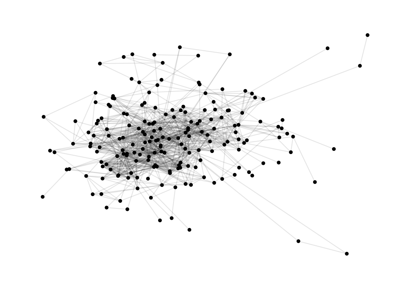
Another cool trick of alpha:
ggraph(lemur, layout = "kk") +
  geom_edge_link(aes(alpha = ..index..), show.legend = FALSE) +
  geom_node_point(size = 4) +
  theme_graph()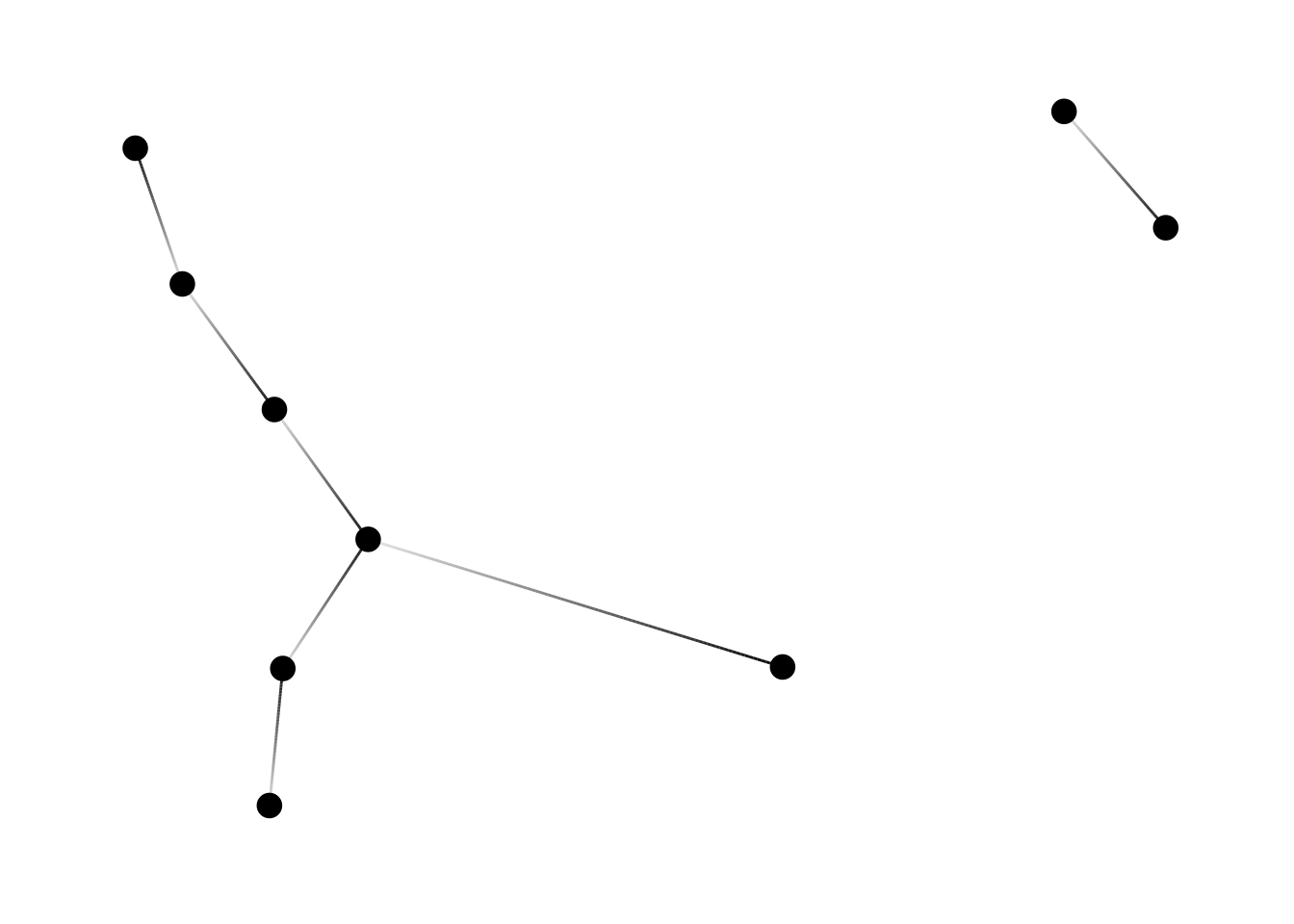
6.1.5 beginning and the end
6.1.5.1 Arrows
We’ll see some arrows:
ggraph(lemur, layout = "kk") +
  geom_edge_link(
    colour = "purple",
    arrow = arrow(length = unit(4, 'mm'))
  ) +
  geom_node_point(size = 4) +
  theme_graph()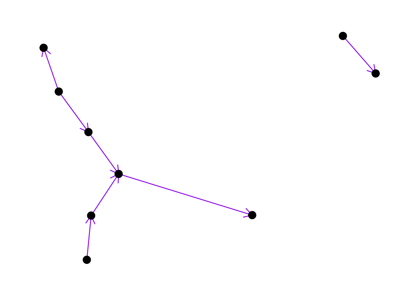
ggraph(lemur, layout = "kk") +
  geom_edge_link(
    colour = "grey",
    arrow = arrow(angle = 45, length = unit(7, 'mm'), type = "closed")
  ) +
  geom_node_point(size = 4) +
  theme_graph()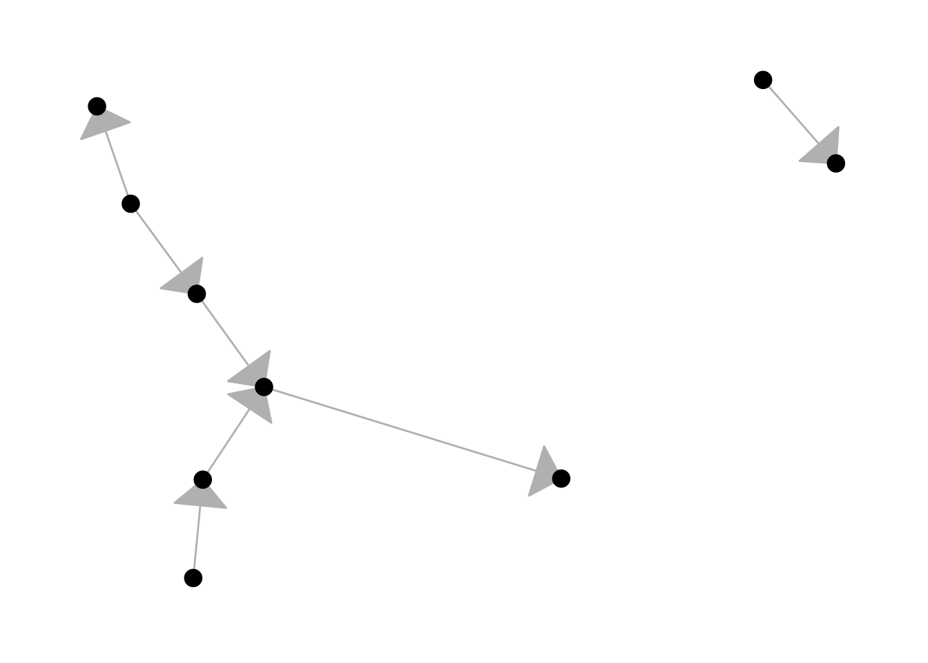
It’s ok, but we would like to avoid overlap between the edges and nodes, which we can achieve by start_cap and end_cap:
ggraph(lemur, layout = "kk") +
  geom_edge_link(
    colour = "grey",
    arrow = arrow(angle = 45, length = unit(4, 'mm'), type = "closed"),
    end_cap = circle(3, 'mm')
  ) +
  geom_node_point(size = 4) +
  theme_graph()
Let’s do the same for the start
ggraph(lemur, layout = "kk") +
  geom_edge_link(
    colour = "grey",
    arrow = arrow(angle = 45, length = unit(4, 'mm'), type = "closed"),
    start_cap = circle(6, 'mm'),
    end_cap = circle(3, 'mm')
  ) +
  geom_node_point(size = 4) +
  theme_graph()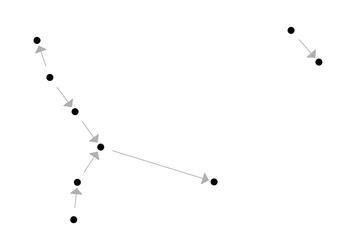
6.2 Different types of edges
Within the package ggraph, we can use the following functions to create different kinds of edges. Some edge types are only useful or particular layouts. :
6.2.1 geom_edge_link
The one we’ve been seeing all along:
ggraph(lemur, layout = "kk") +
  geom_edge_link() +
  geom_node_point(size = 4) +
  theme_graph()
6.2.2 geom_edge_arc
Bendy bendy, so overlapping lines are visible.
ggraph(lemur, layout = "kk") +
  geom_edge_arc() +
  geom_node_point(size = 4) +
  theme_graph()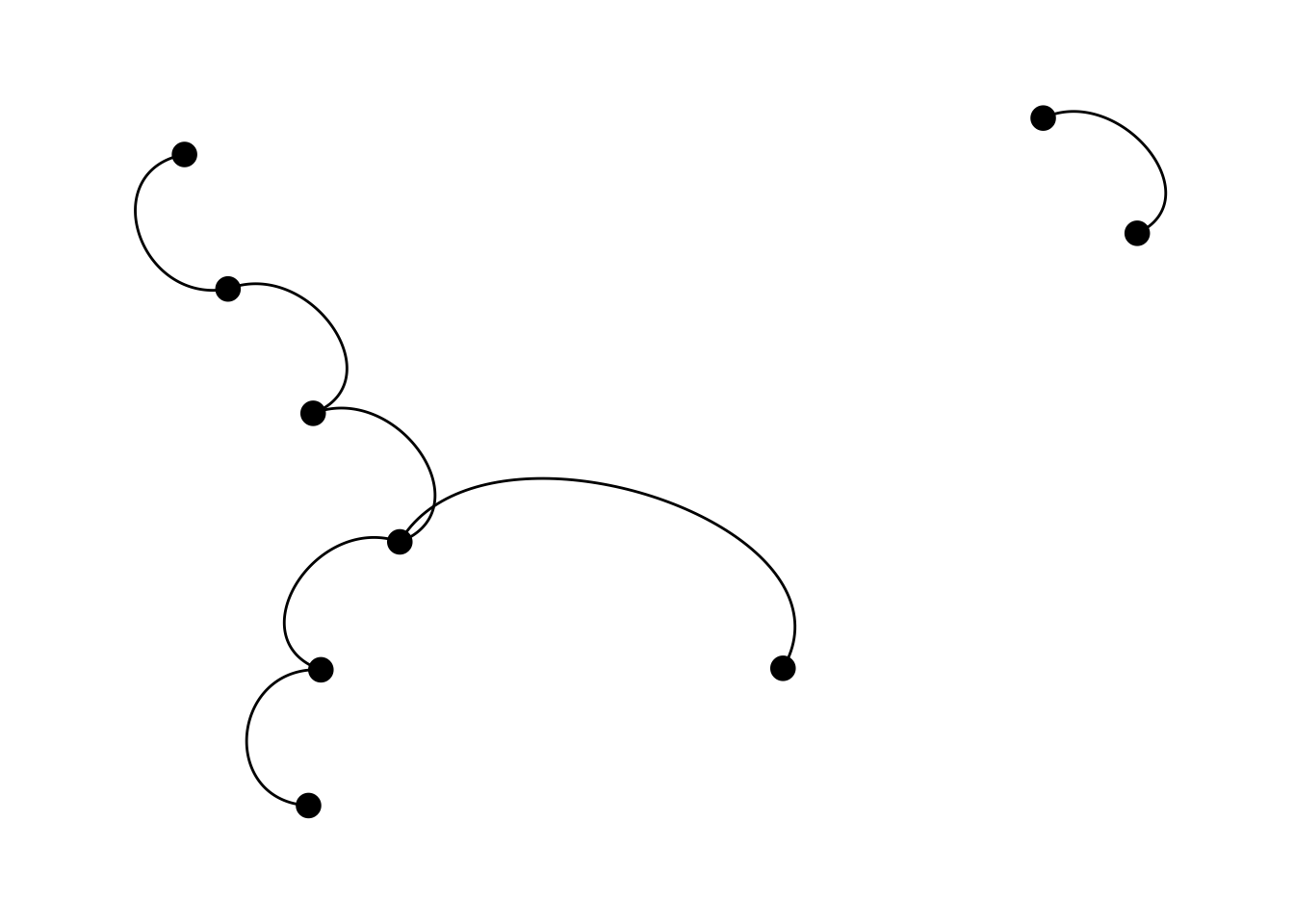
In the above case they’re not so useful, let’s find a better example:
ggraph(lemur, layout = "linear") +
  geom_edge_arc(colour = "grey") +
  geom_node_point(size = 4) +
  theme_graph()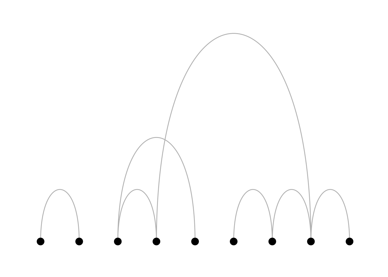
ggraph(lemur, layout = "linear", circular = TRUE) +
  geom_edge_arc(colour = "grey") +
  geom_node_point(size = 4) +
  theme_graph() +
  coord_fixed()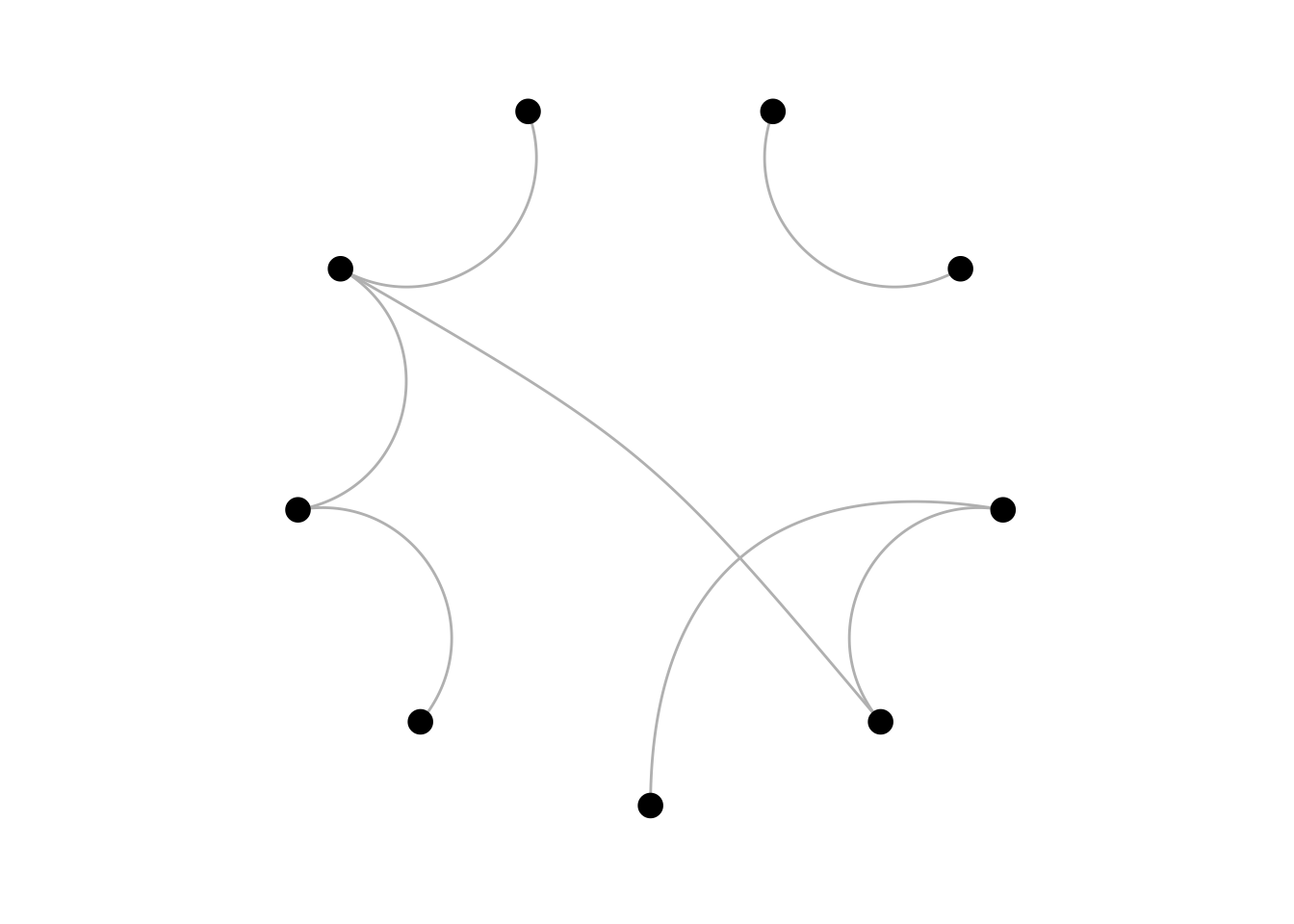
6.2.3 geom_edge_bend
Particularly useful for hierarchical plots.
ggraph(lemur, layout = "tree") +
  geom_edge_bend() +
  geom_node_point(size = 4) +
  theme_graph()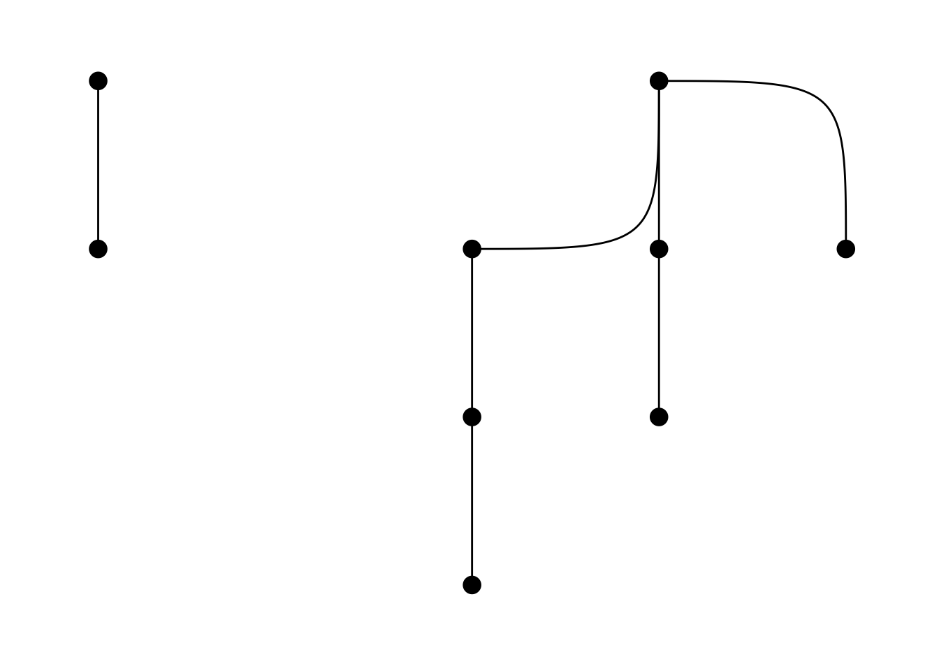
6.2.4 geom_edge_diagonal
Also useful for hierarchical plots
ggraph(lemur, layout = "tree") +
  geom_edge_diagonal() +
  geom_node_point(size = 4) +
  theme_graph()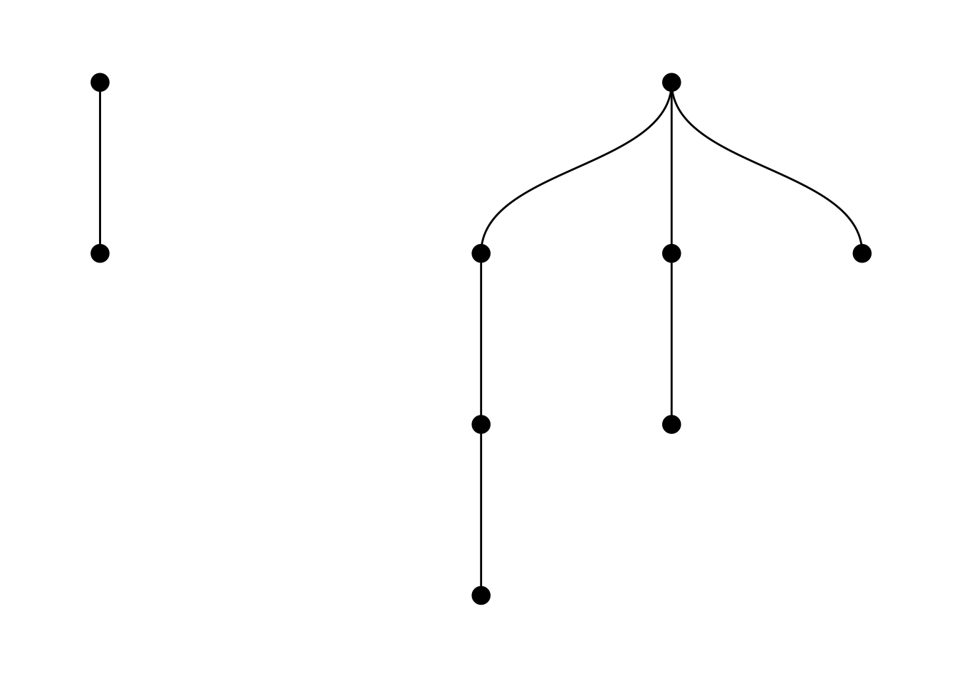
6.2.5 geom_edge_fan
The fan is useful when you have directed arrows between two nodes. Let’s revise our data on lemur by drawing additional directional ties. We’ll draw a tie from 2 to 1, rom 8 to 7, and from 1 to 1:
lemur2 <- lemur %>%
  convert(to_directed) %>%
  bind_edges(data.frame(from = c(2, 8, 1), to = c(1, 7, 1), weight = c(1, 1, 1)))

lemur2 %>% activate(edges) %>% arrange(from)
## # A tbl_graph: 9 nodes and 10 edges
## #
## # A directed multigraph with 2 components
## #
## # Edge Data: 10 × 4 (active)
## from to weight .tidygraph_edge_index
## <int> <int> <dbl> <int>
## 1 1 2 1 1
## 2 1 1 1 NA
## 3 2 1 1 NA
## 4 3 4 1 2
## 5 3 5 1 3
## 6 4 8 1 4
## # … with 4 more rows
## #
## # Node Data: 9 × 4
## `residence status` SEX id .tidygraph_node_index
## <chr> <chr> <chr> <int>
## 1 "immigrant" MALE A 1
## 2 "resident" FEMALE TR 2
## 3 "" MALE G 3
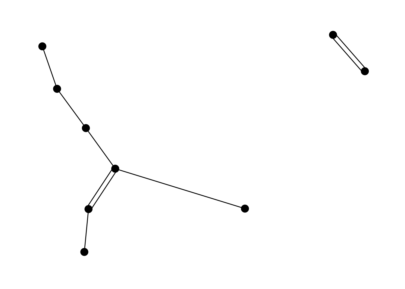
## # … with 6 more rowsWith geom_edge_link we don’t see the directed ties!
ggraph(lemur2, layout = "kk") +
  geom_edge_link() +
  geom_node_point(size = 4) +
  theme_graph()
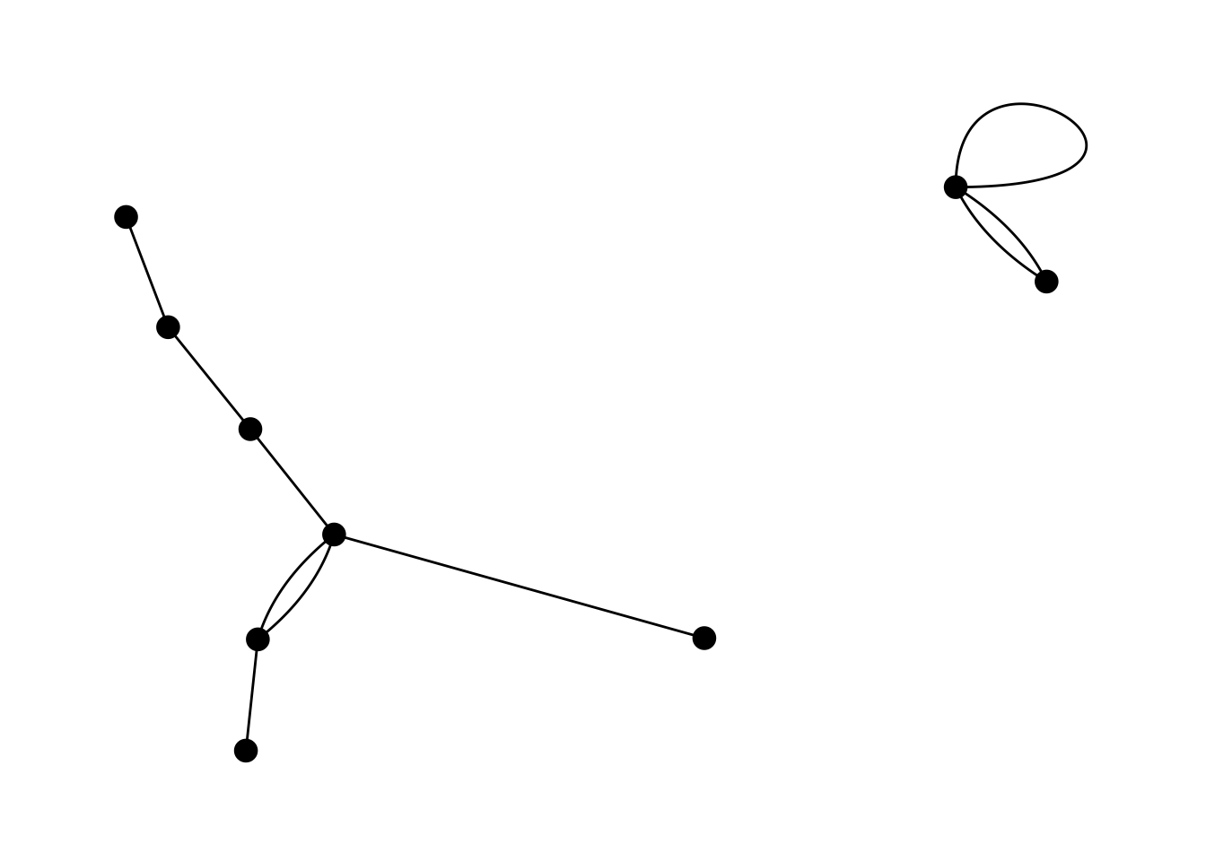
geom_edge_fan to save the day.
ggraph(lemur2, layout = "kk") +
  geom_edge_fan() +
  geom_node_point(size = 4) +
  theme_graph()
6.3 DIY
Try to make something fancy for the Zebras! Data from this wonderful website.

zebra_graphml <- read.graph("https://raw.githubusercontent.com/bansallab/asnr/master/Networks/Mammalia/zebra_groupmembership_weighted/zebra_sundaresan_interaction_attribute.graphml", format = "graphml")

zebra <- as_tbl_graph(zebra_graphml)