Chapter 5 layouts

5.1 choosing a layout

Depending on what you want to show, different layouts help you in achieving that goal. The list of layouts in igraph is:

ggpraph(data, layout = "[insert name algorithm]") ...

name	explanation	when
bipartite	[Simple two-row layout for bipartite graphs]	two independent groups
circle	[circle shaped]	equal importance of nodes, equal distances facilitate communication, small networks
dh	[Davidson-Harel layout algorithm]	force-directed layout that lead to closely connected nodes being closer to one another, loosely connected nodes pushed towards outside
drl	[DrL graph layout generator]	force-directed layout for large graphs that lead to closely connected nodes being closer to one another, loosely connected nodes pushed towards outside
fr	[Fruchterman-Reingold layout algorithm]	force-directed layout that lead to closely connected nodes being closer to one another, loosely connected nodes pushed towards outside
grid	[simple grid layout]	small networks, fixed layout easy to interpret
gem	[GEM layout algorithm]	force-directed layout that lead to closely connected nodes being closer to one another, loosely connected nodes pushed towards outside
graphopt	[graphopt layout algorithm]	force-directed layout for large graphs that lead to closely connected nodes being closer to one another, loosely connected nodes pushed towards outside
kk	[Kamada-Kawai layout algorithm]	force-directed layout that lead to closely connected nodes being closer to one another, loosely connected nodes pushed towards outside
lgl	[Large Graph Layout]	force-directed layout for very large graphs that lead to closely connected nodes being closer to one another, loosely connected nodes pushed towards outside
mds	[layout by multidimensional scaling]	when you want to use multiple measures of distance between nodes to determine layout
nicely	[picks one for you based on data]	useful start
randomly	[random placement]	never
sugiyama	[Sugiyama graph layout generator]	layered/hierarchical network where there is an ordered sequence of events/actions/relationships. Designed for layered directed acyclic graphs, and minimises edge crossings
sphere	[sphere shaped]	not sure, small networks
star	[star shaped]	not sure, small networks
tree	[Reingold-Tilford graph layout algorithm]	hierarchical network (tree!)

Let’s load in some data.

df_edges <- data.frame(
  from = c("Gert","Gert","Gert","Gert","Gert","Ben","Anne"),
  to = c("Anne","Ben","Winy","Vera","Laura","Winy","Vera"),
  closeness = c("very close", "close", "close", "close", "somewhat close", 
                "very close", "very close")
)

df_nodes <- data.frame(
  name = c("Gert", "Anne", "Ben", "Winy", "Vera", "Laura"),
  relation = c("Ego", "Partner", "Family", "Family", "Friend", "Friend")
)

df_network <- tbl_graph(nodes = df_nodes, edges = df_edges, directed = FALSE)

It’s a small network, let’s try a circle:

ggraph(df_network, layout = "circle") +
  geom_edge_link(aes(linetype = closeness)) +
  geom_node_point(aes(colour = relation), size = 13) +
  geom_node_text(aes(label = name), colour = "white") +
  theme_void() +
  scale_color_brewer(palette = "Set2")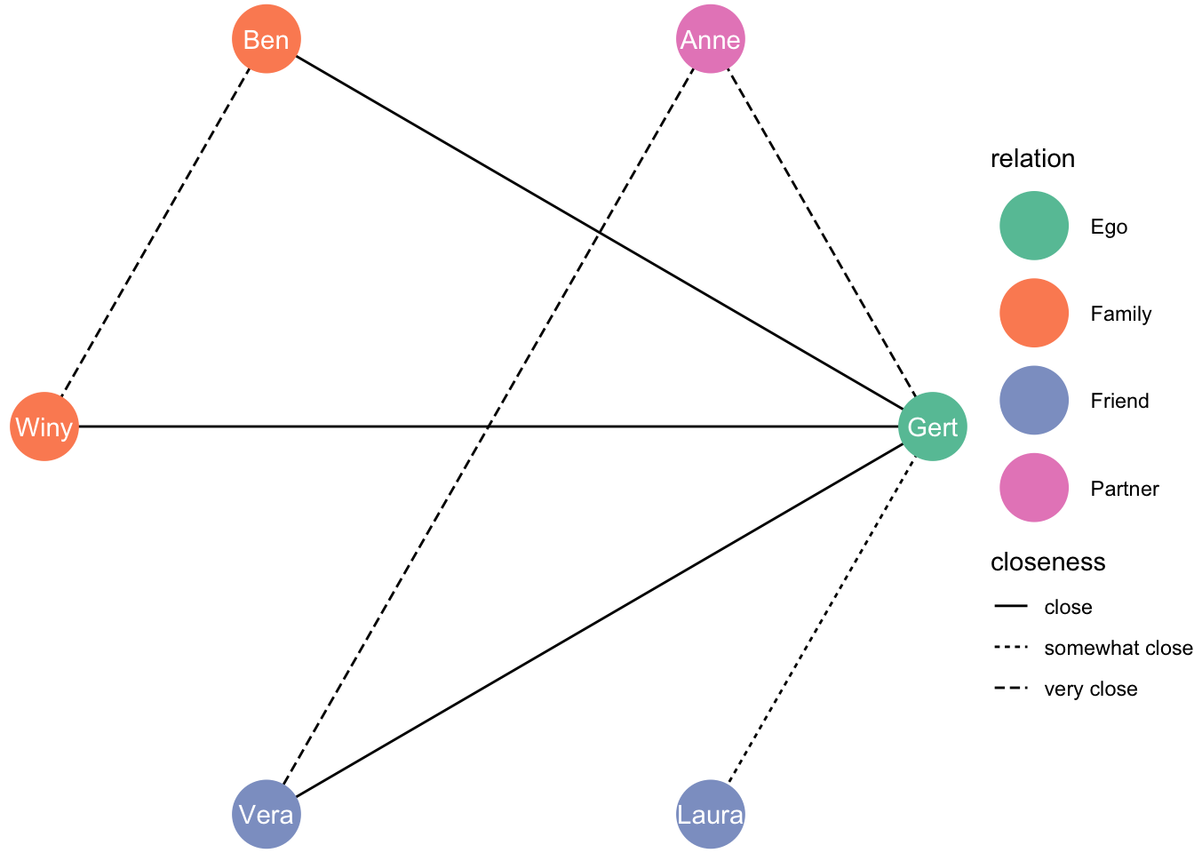

5.1.0.1 Circle with ego in the middle!

[this layout comes from the package graphlayouts]

ggraph(df_network, layout = "focus", focus = 1) +
  geom_edge_link(aes(linetype = closeness)) +
  geom_node_point(aes(colour = relation), size = 13) +
  geom_node_text(aes(label = name), colour = "white") +
  theme_void() +
  scale_color_brewer(palette = "Set2")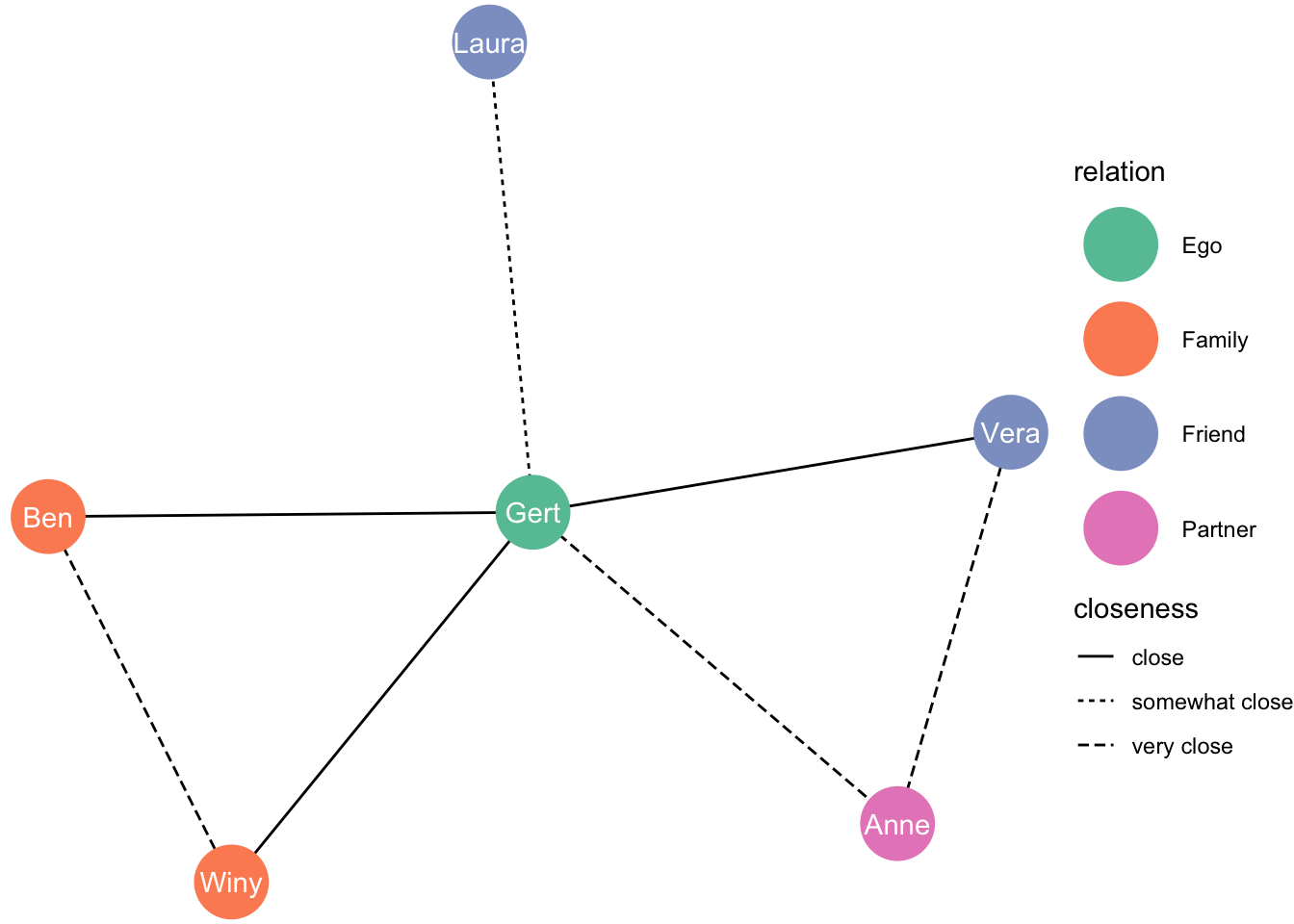

Or on a square?

ggraph(df_network, layout = "grid") +
  geom_edge_link(aes(linetype = closeness)) +
  geom_node_point(aes(colour = relation), size = 13) +
  geom_node_text(aes(label = name), colour = "white") +
  theme_void() +
  scale_color_brewer(palette = "Set2")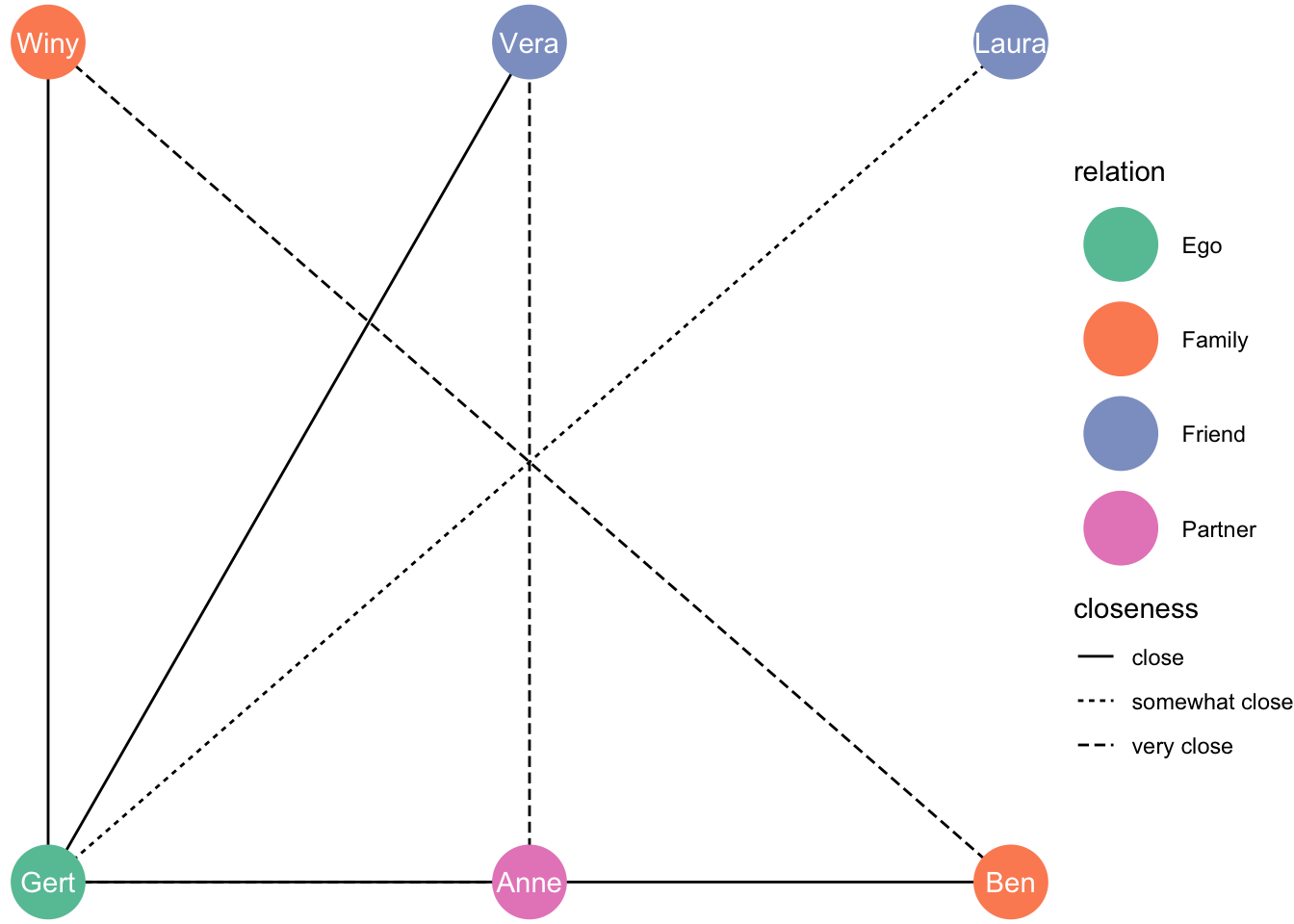

Using a force-directed algorithm (Fruchterman-Reingold layout algorithm) :

set.seed(1)
ggraph(df_network, layout = "fr") +
  geom_edge_link(aes(linetype = closeness)) +
  geom_node_point(aes(colour = relation), size = 13) +
  geom_node_text(aes(label = name), colour = "white") +
  theme_void() +
  scale_color_brewer(palette = "Set2")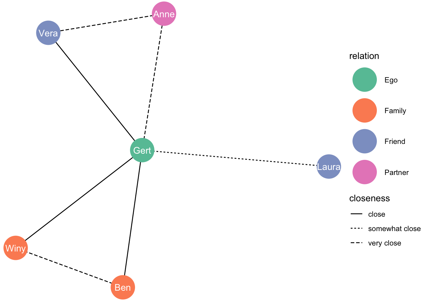

Slightly different each time:

set.seed(2)
ggraph(df_network, layout = "fr") +
  geom_edge_link(aes(linetype = closeness)) +
  geom_node_point(aes(colour = relation), size = 13) +
  geom_node_text(aes(label = name), colour = "white") +
  theme_void() +
  scale_color_brewer(palette = "Set2")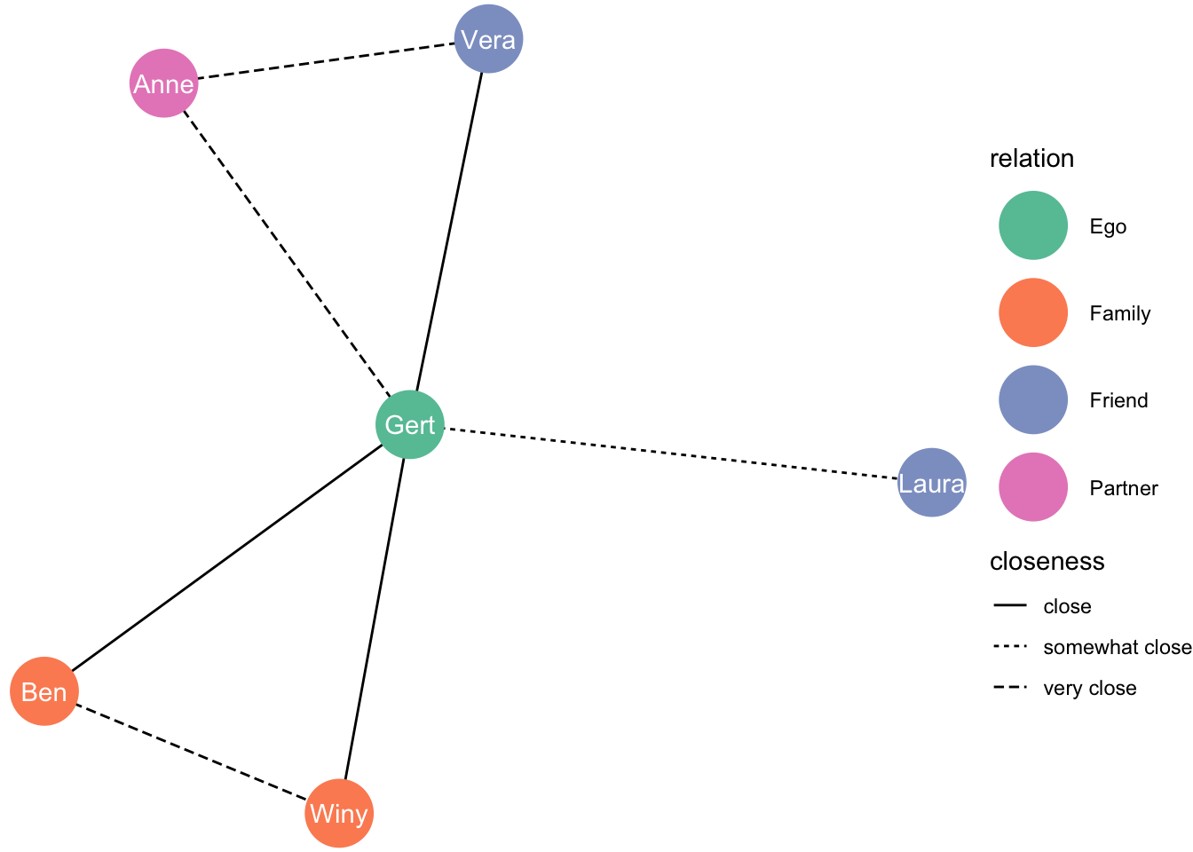

Let’s look at larger graphs on … dolphins! 190 of them. First the data.

library(igraph)
dolphins_graphml <- igraph::read.graph("https://raw.githubusercontent.com/bansallab/asnr/master/Networks/Mammalia/dolphin_association_weighted/weighted_FORAGE_dolphin_florida.graphml", format = "graphml")

dolphins <- as_tbl_graph(dolphins_graphml)

Let’s try putting them in a circle.

ggraph(dolphins, layout = "circle") +
  geom_edge_link() +
  geom_node_point() +
  theme_graph() +
  coord_fixed()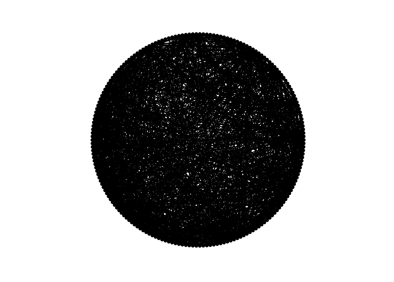

Ok…

ggraph(dolphins, layout = "circle") +
  geom_edge_link(alpha = 0.1) +
  geom_node_point() +
  theme_graph() +
  coord_fixed()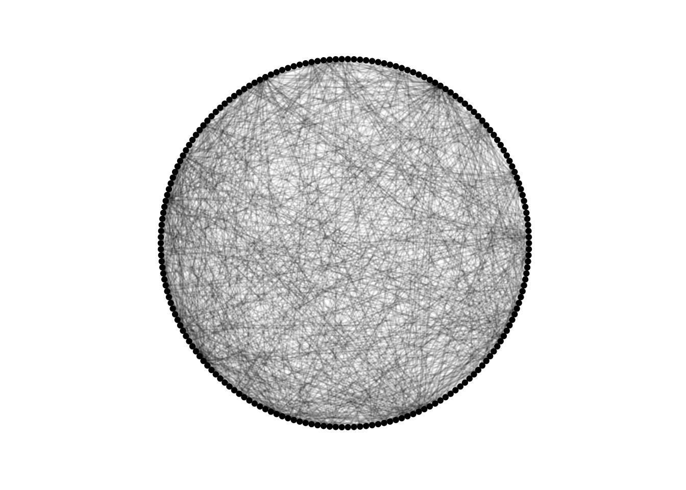

Pretty but useless!

Let’s try these force-directed layouts that handle large networks better.

ggraph(dolphins, layout = "kk") +
  geom_edge_link() +
  geom_node_point() +
  theme_graph()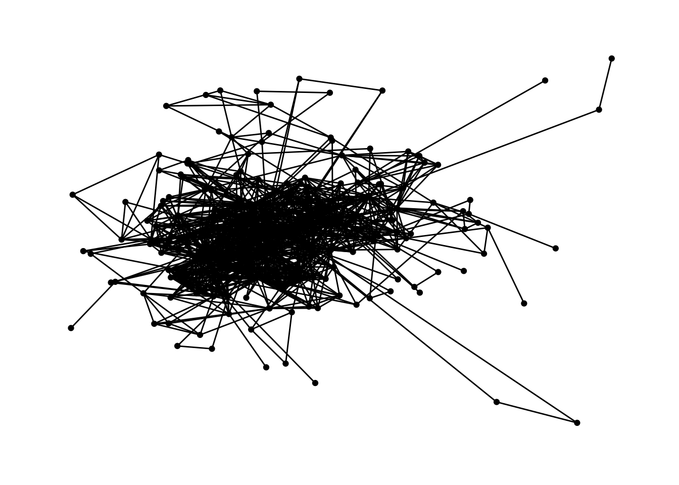 

The many edges make these graphs problematic. Some layout alghorithms reduced the number of edges/ties. We opt for making them very light in colour, and see through:

ggraph(dolphins, layout = "kk") +
  geom_edge_link(alpha = 0.1) +
  geom_node_point() +
  theme_graph()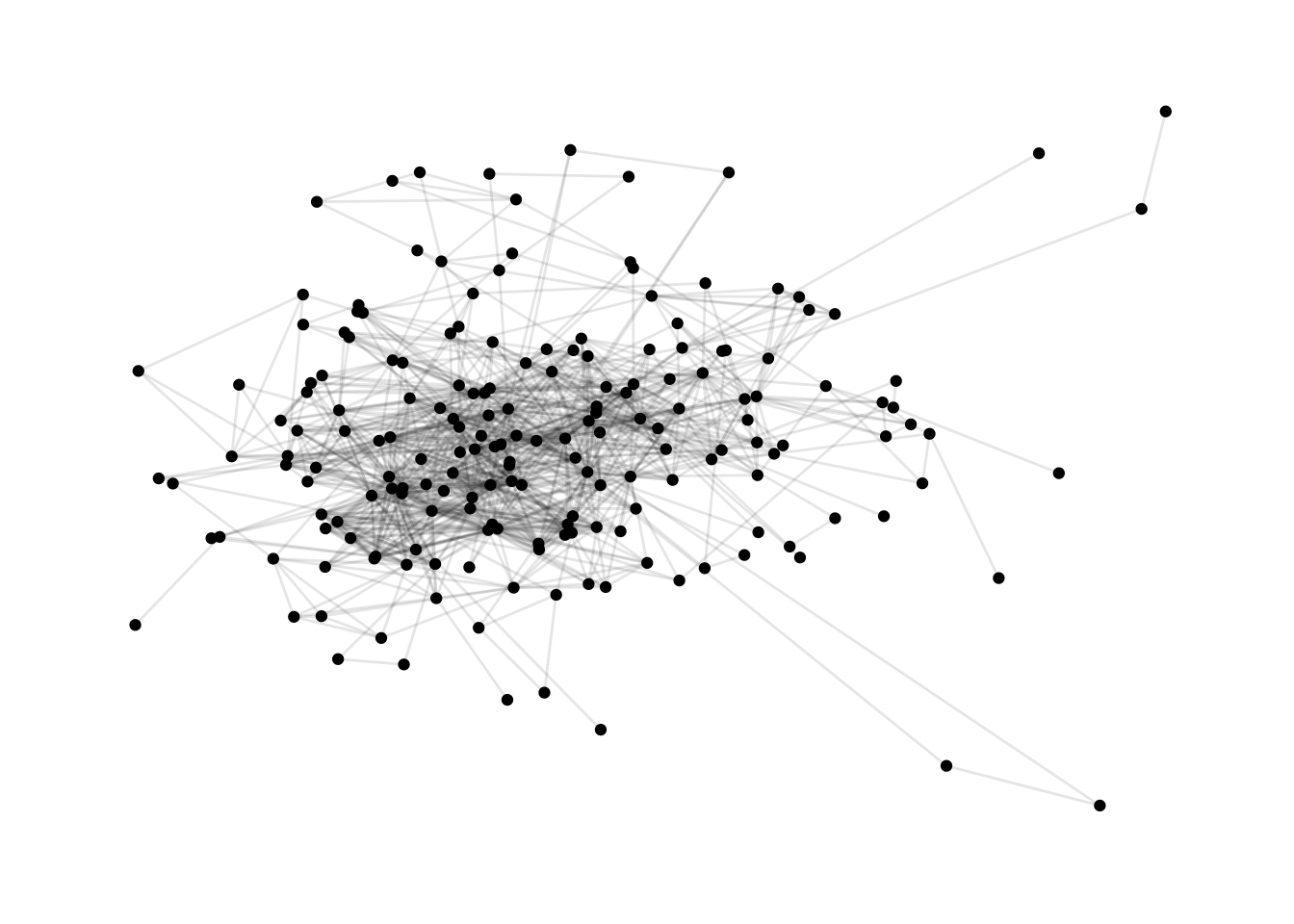 

ggraph(dolphins, layout = "fr") +
  geom_edge_link(alpha = 0.1) +
  geom_node_point() +
  theme_graph()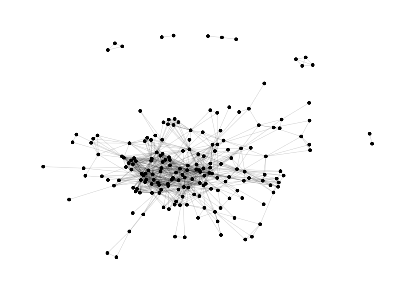 

ggraph(dolphins, layout = "dh") +
  geom_edge_link(alpha = 0.1) +
  geom_node_point() +
  theme_graph()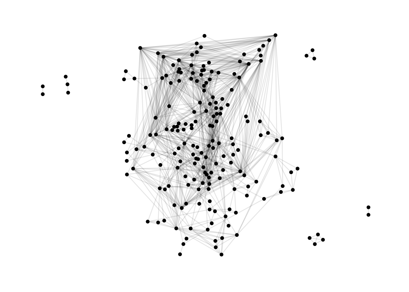 

5.1.1 Keeping a layout for future use

Remember this graph?

set.seed(1)
ggraph(df_network, layout = "fr") +
  geom_edge_link(aes(linetype = closeness)) +
  geom_node_point(aes(colour = relation), size = 13) +
  geom_node_text(aes(label = name), colour = "white") +
  theme_void() +
  scale_color_brewer(palette = "Set2")

Let’s say I have also information on the frequency of contact, and I also would like to show this information in a graph, then it would be useful to have exactly the same layout. Let’s see how to do this:

First, let’s create the new information on frequency of contact:

df_network <- df_network  %>% 
  activate(edges) %>% 
  mutate( # Create new variable in edges dataset
    freq_cont = c("daily", "monthly", "monthly", "monthly", "weekly",
                  "daily", "monthly")
  )

We’ve indeed managed to create new variable:

df_network

## # A tbl_graph: 6 nodes and 7 edges
## #
## # An undirected simple graph with 1 component
## #
## # Edge Data: 7 × 4 (active)
##    from    to closeness      freq_cont
##   <int> <int> <chr>          <chr>    
## 1     1     2 very close     daily    
## 2     1     3 close          monthly  
## 3     1     4 close          monthly  
## 4     1     5 close          monthly  
## 5     1     6 somewhat close weekly   
## 6     3     4 very close     daily    
## # … with 1 more row
## #
## # Node Data: 6 × 2
##   name  relation
##   <chr> <chr>   
## 1 Gert  Ego     
## 2 Anne  Partner 
## 3 Ben   Family  
## # … with 3 more rows

Now, we want two graphs with the same layout, one for closeness, and one for frequency of contact. We need to keep the layout that the algorithm that determined our layout is kept:

set.seed(1)
layout_nw <- create_layout(df_network, layout = 'fr')

Just a simple dataframe:

layout_nw

##          x        y  name relation .ggraph.orig_index circular .ggraph.index
## 1 7.689453 11.83531  Gert      Ego                  1    FALSE             1
## 2 7.858226 13.19301  Anne  Partner                  2    FALSE             2
## 3 7.539544 10.47034   Ben   Family                  3    FALSE             3
## 4 6.709893 10.86258  Winy   Family                  4    FALSE             4
## 5 6.962720 13.00292  Vera   Friend                  5    FALSE             5
## 6 9.134448 11.67227 Laura   Friend                  6    FALSE             6

Let’s graph:

closeness_graph <- ggraph(layout_nw) +
  geom_edge_link(aes(linetype = closeness)) +
  geom_node_point(aes(colour = relation), size = 13) +
  geom_node_text(aes(label = name), colour = "white") +
  theme_void() +
  scale_color_brewer(palette = "Set2")

closeness_graph

Now let’s graph frequency of contact

freq_cont_graph <- ggraph(layout_nw) +
  geom_edge_link(aes(linetype = freq_cont)) +
  geom_node_point(aes(colour = relation), size = 13) +
  geom_node_text(aes(label = name), colour = "white") +
  theme_void() +
  scale_color_brewer(palette = "Set2")

freq_cont_graph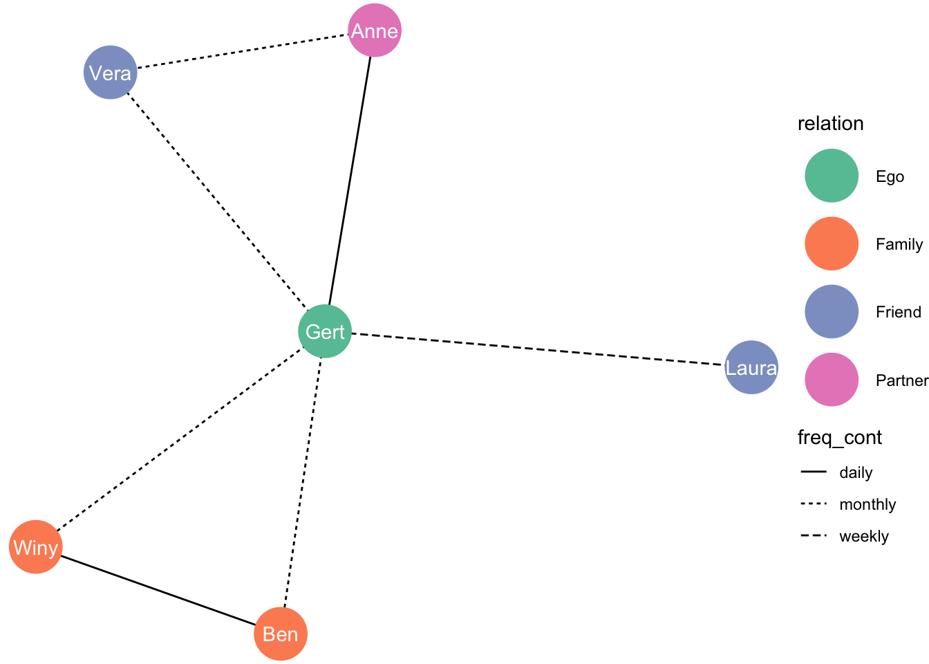

Let’s put them next to one another:

library(patchwork)
closeness_graph + freq_cont_graph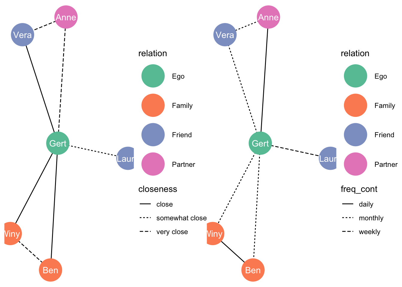

5.2 DIY

Here is data from Zebra!

zebra_graphml <- read.graph("https://raw.githubusercontent.com/bansallab/asnr/master/Networks/Mammalia/zebra_groupmembership_weighted/zebra_sundaresan_interaction_attribute.graphml", format = "graphml")

zebra <- as_tbl_graph(zebra_graphml)

Try to find a useful layout

5.3 Further reading

This, this, and this is useful.