Facets

An amazing features of ggplot, is facetting. Rather than explaining what they are, I will just show you:

ggplot(mpg, aes(x = cty)) + geom_histogram(binwidth = 1) + facet_wrap(~manufacturer)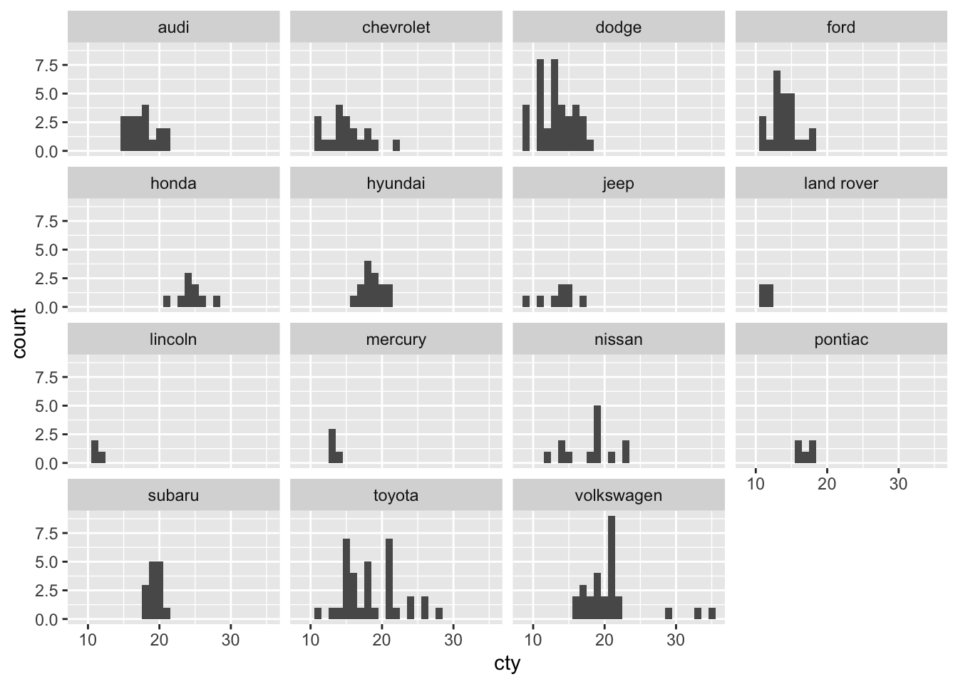

Facetting groups the data and displays the data for each group. This allows for comparing multiple groups readily. Let’s see some other examples. Remember this graph:

ggplot(mpg, aes(x = displ, y = cty, colour = drv)) +
  geom_point() +
  geom_smooth(method = "lm", se = FALSE)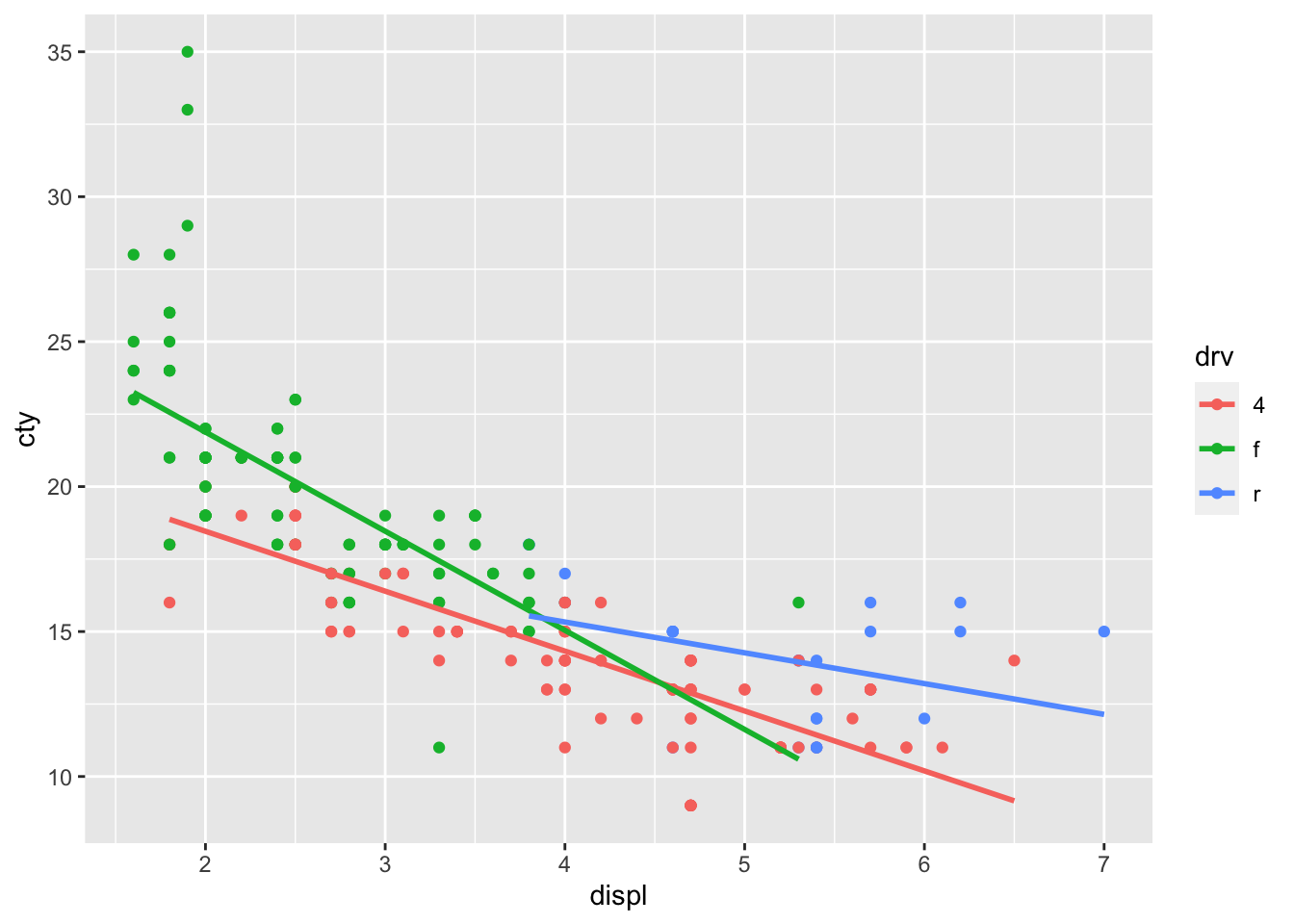

With facets:

ggplot(mpg, aes(x = displ, y = cty)) +
  geom_point() +
  geom_smooth(method = "lm", se = FALSE) +
  facet_wrap(~drv)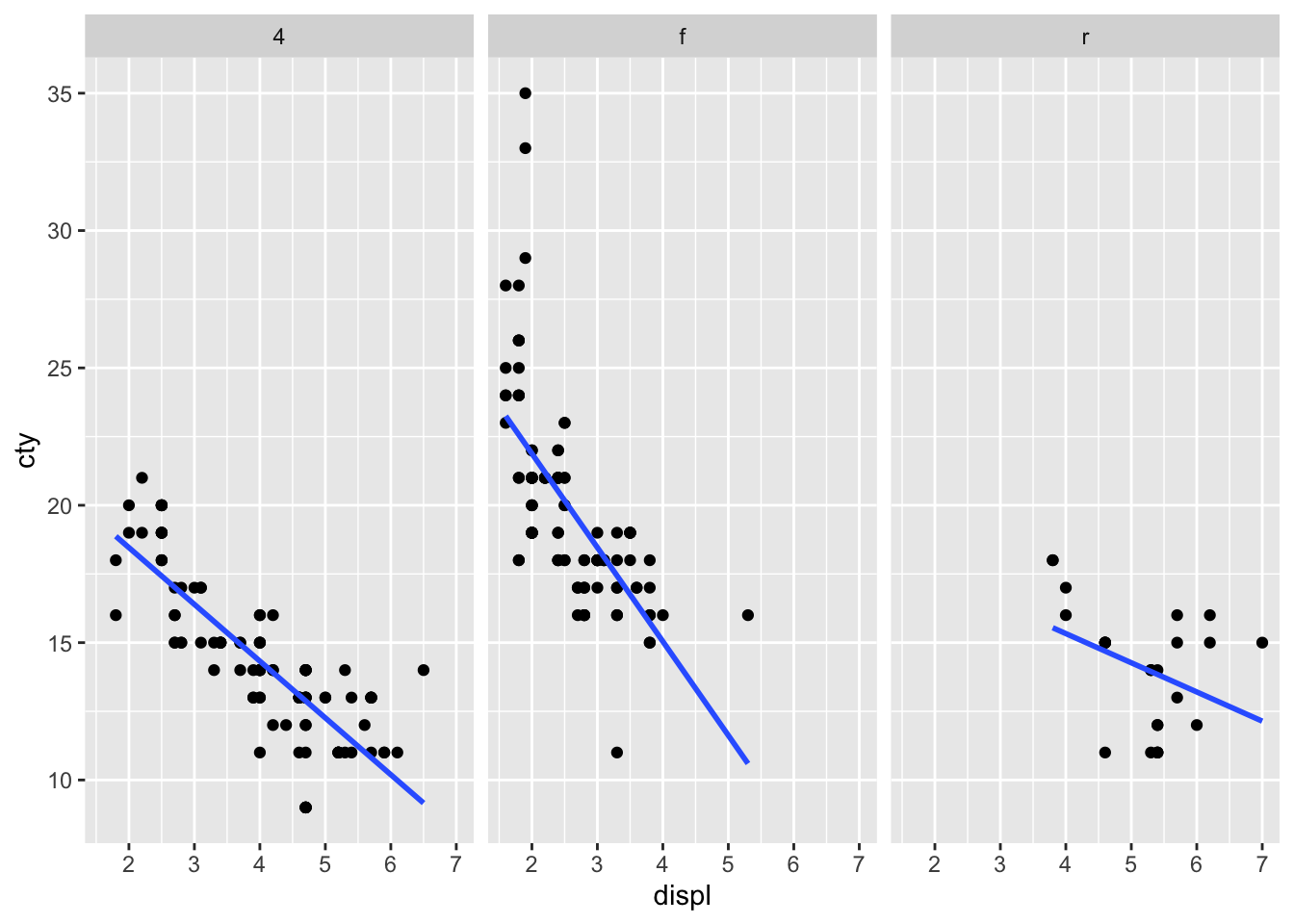

We can also put them under one another:

ggplot(mpg, aes(x = displ, y = cty)) +
  geom_point() +
  geom_smooth(method = "lm", se = FALSE) +
  facet_wrap(~drv, nrow = 3)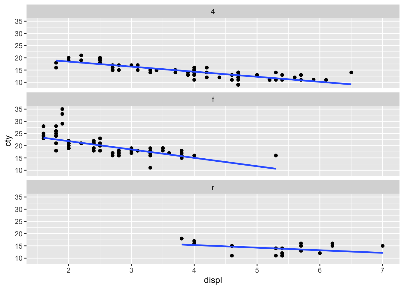

Or use multiple variables with facet_grid

ggplot(mpg, aes(x = displ, y = cty)) +
  geom_point() +
  geom_smooth(method = "lm", se = FALSE) +
  facet_grid(year ~ drv)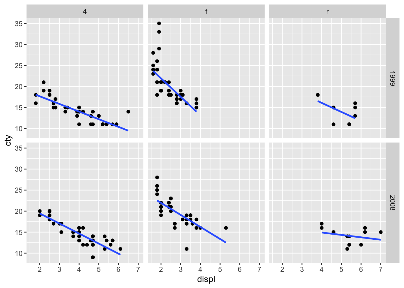

Cool trick

One neat little trick is to have the raw data present in each facet. You can do this by using a dataframe that does NOT include the facetting variable. The data = transform(mpg, drv = NULL) below means for this geom we will use a different dataset, which is the mpg-dataset with the drv-variable set to NULL):

ggplot(mpg, aes(x = displ, y = cty)) +
  geom_point(
    data = transform(mpg, drv = NULL),
    colour = "grey85"
  ) +
  geom_point() +
  geom_smooth(method = "lm", se = FALSE) +
  facet_wrap(~drv)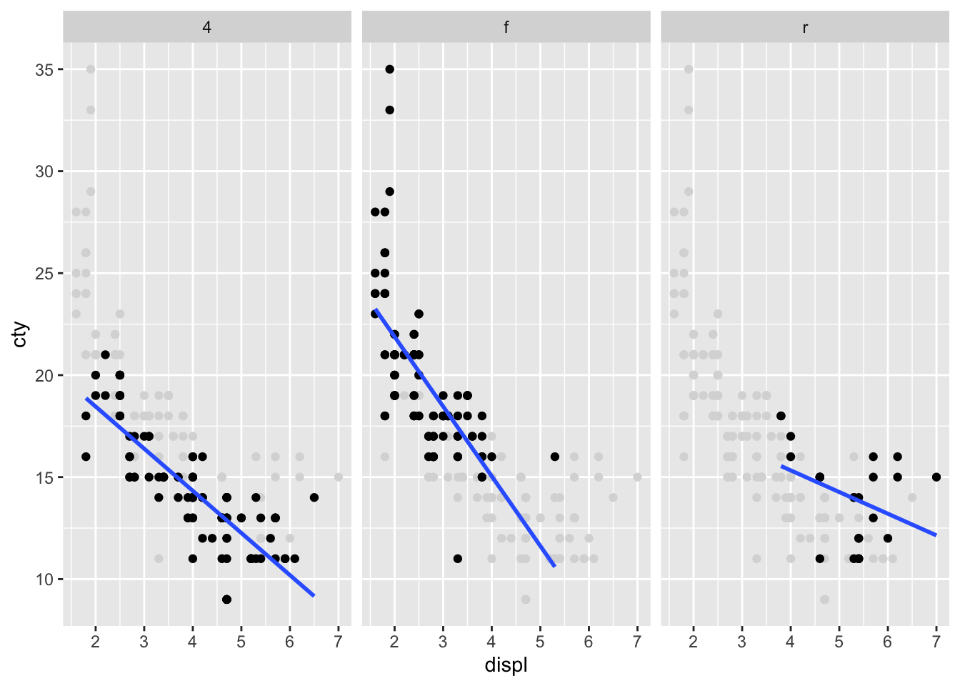

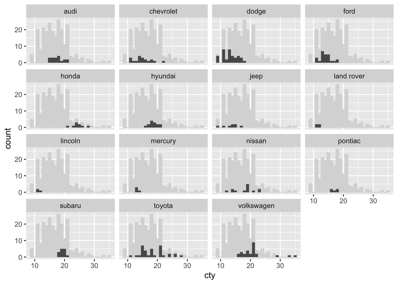
This also works beautifully for histograms:

ggplot(mpg, aes(x = cty)) +
  geom_histogram(
    data = transform(mpg, manufacturer = NULL), fill = "grey85",
    colour = "grey85", binwidth = 1
  ) +
  geom_histogram(binwidth = 1) +
  facet_wrap(~manufacturer)