Chapter 21 Combining plots

Oftentimes you like to present two graphs next to one another. Some packages exist that are helpful in combining multiple graphs in a neatly outlined set of graphs. We’ll focus on patchwork and cowplot. The former is easiest to use, the latter has more options.

21.1 patchwork

patchwork is a great package. For documentation, see here.

install.packages("patchwork")
library(patchwork)

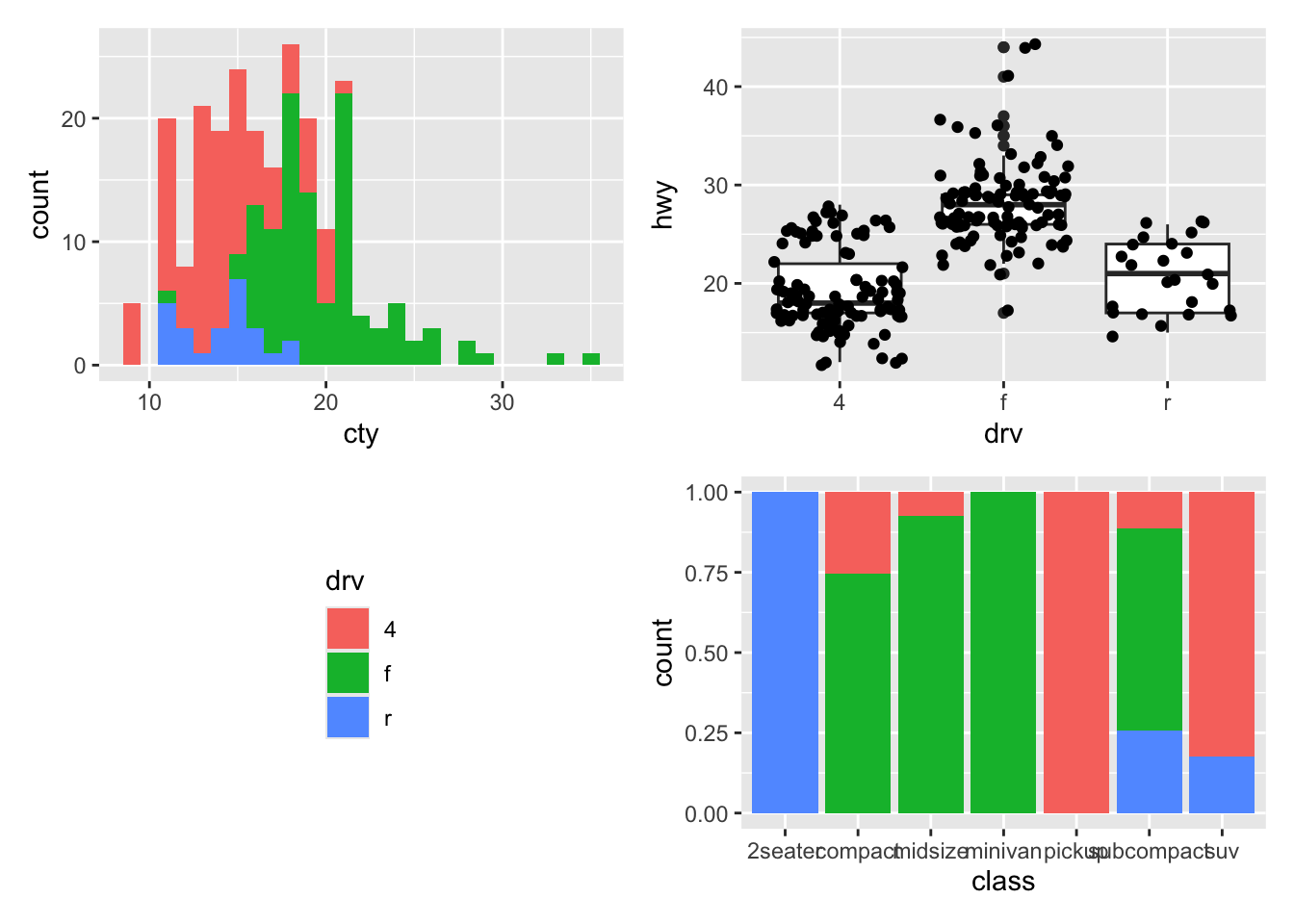
Let’s combine three wildly different graphs:

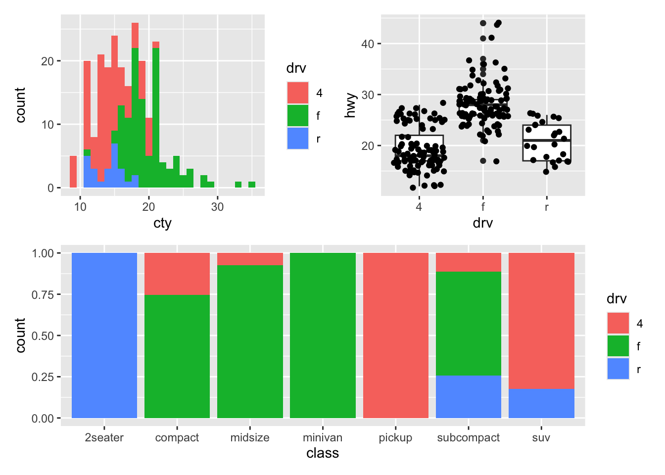
graph1 <- ggplot(mpg, aes(x = cty, fill = drv)) +
  geom_histogram(binwidth = 1)
graph2 <- ggplot(mpg, aes(x = drv, y = hwy)) +
  geom_boxplot() +
  geom_jitter()
graph3 <- ggplot(mpg, aes(x = class, fill = drv)) +
  geom_bar(position = "fill")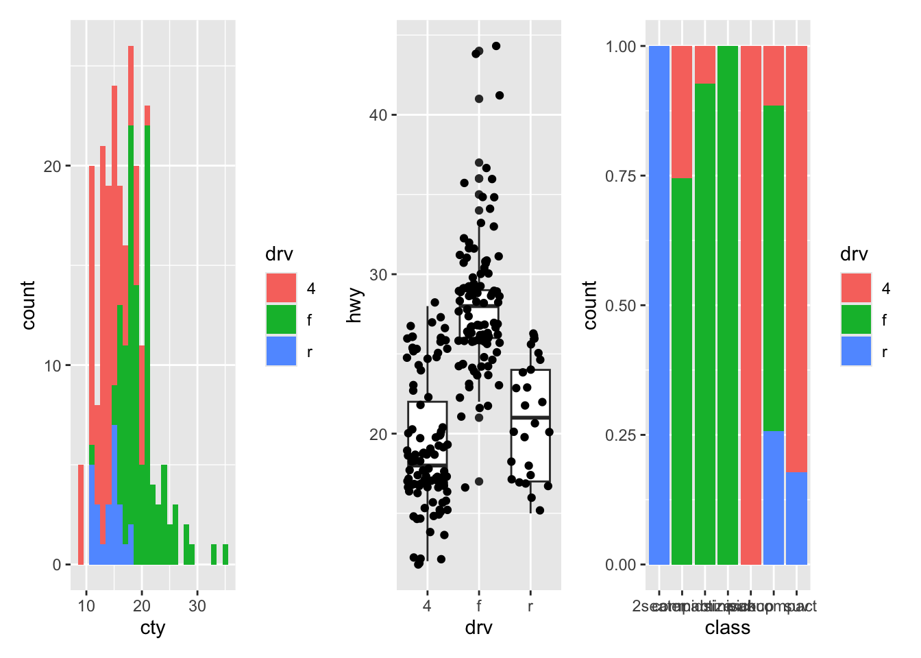

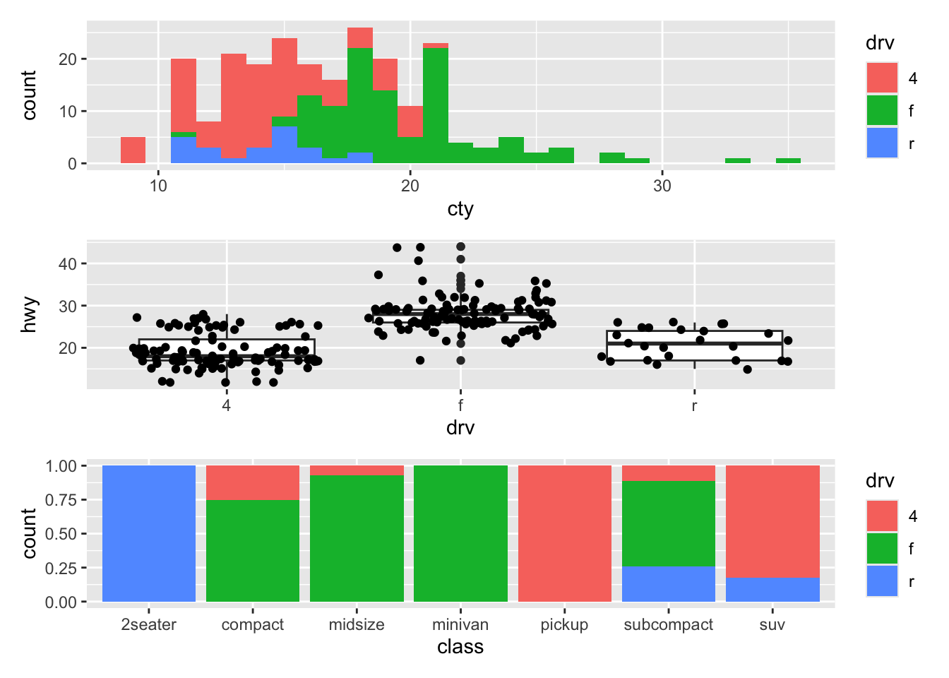
graph1 + graph2 + graph3

graph1 + graph2 + graph3 + plot_layout(nrow = 3)

graph1 + graph2 + graph3 + plot_layout(nrow = 3, height = c(3, 2, 1))

Changing the themes of all with &:

graph1 + graph2 + graph3 +
  plot_layout(nrow = 3, height = c(3, 2, 1)) &
  theme_minimal()

Let’s add a fourth “graph” which is text:

graph1 + graph2 + graph3 + grid::textGrob("This is not really a fourth graph")

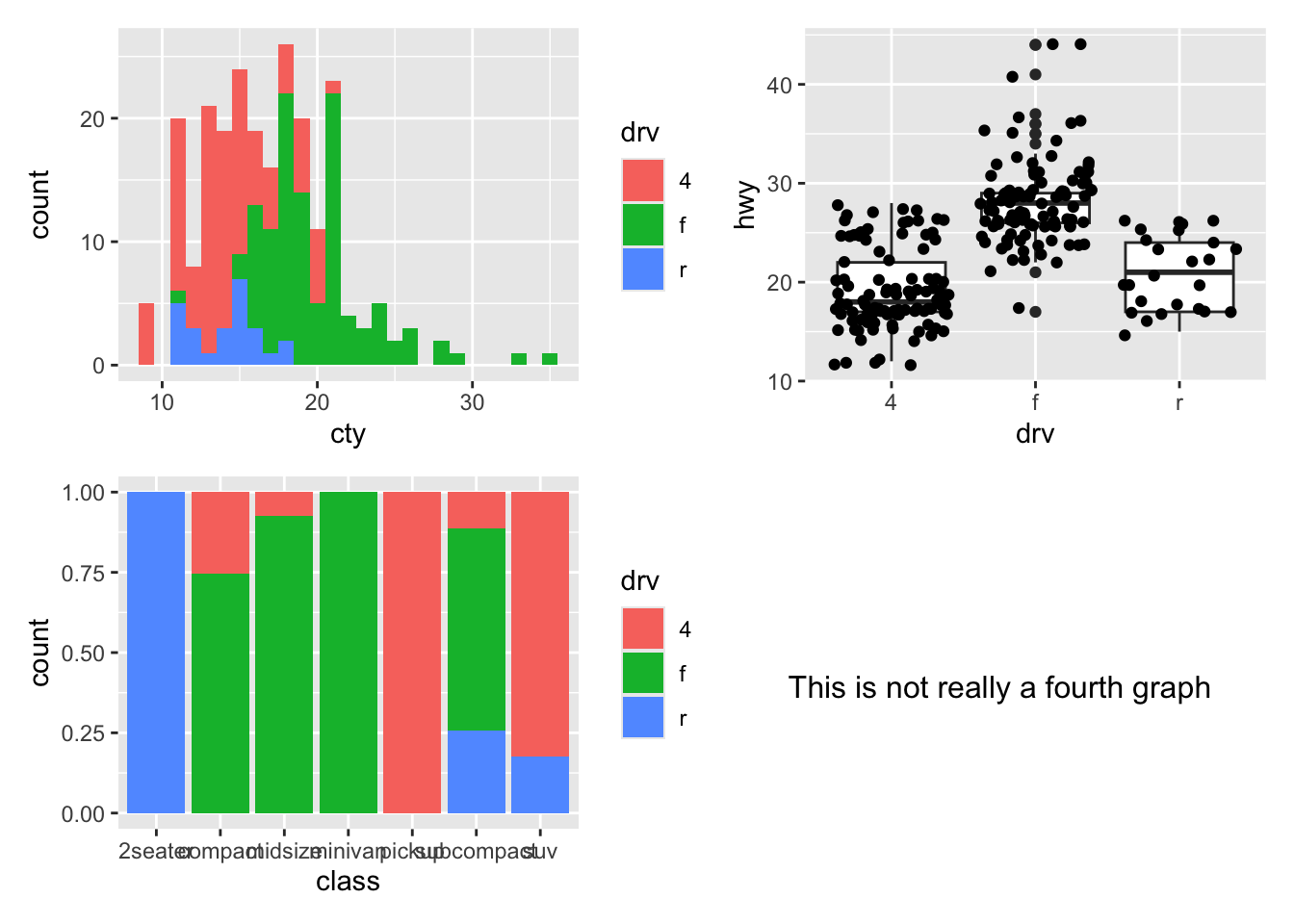
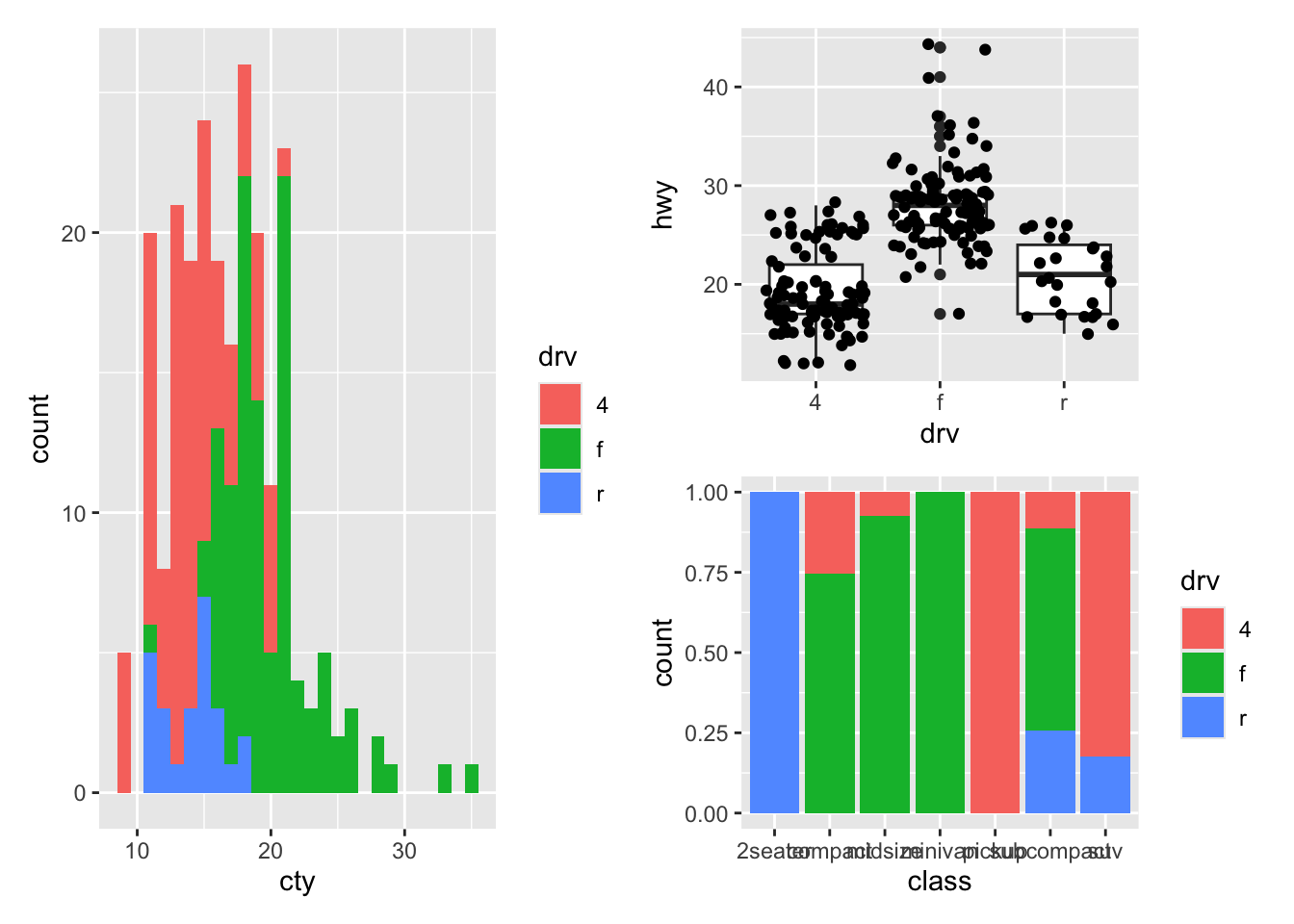
patchwork provides 2 shortcut operators: | places plots next to each other while / place them on top of each other. Brackets help you in making the layout:

(graph1 | graph2) / graph3

graph1 | (graph2 / graph3)

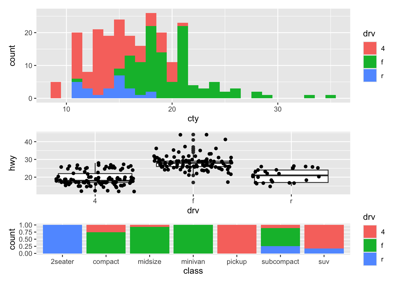
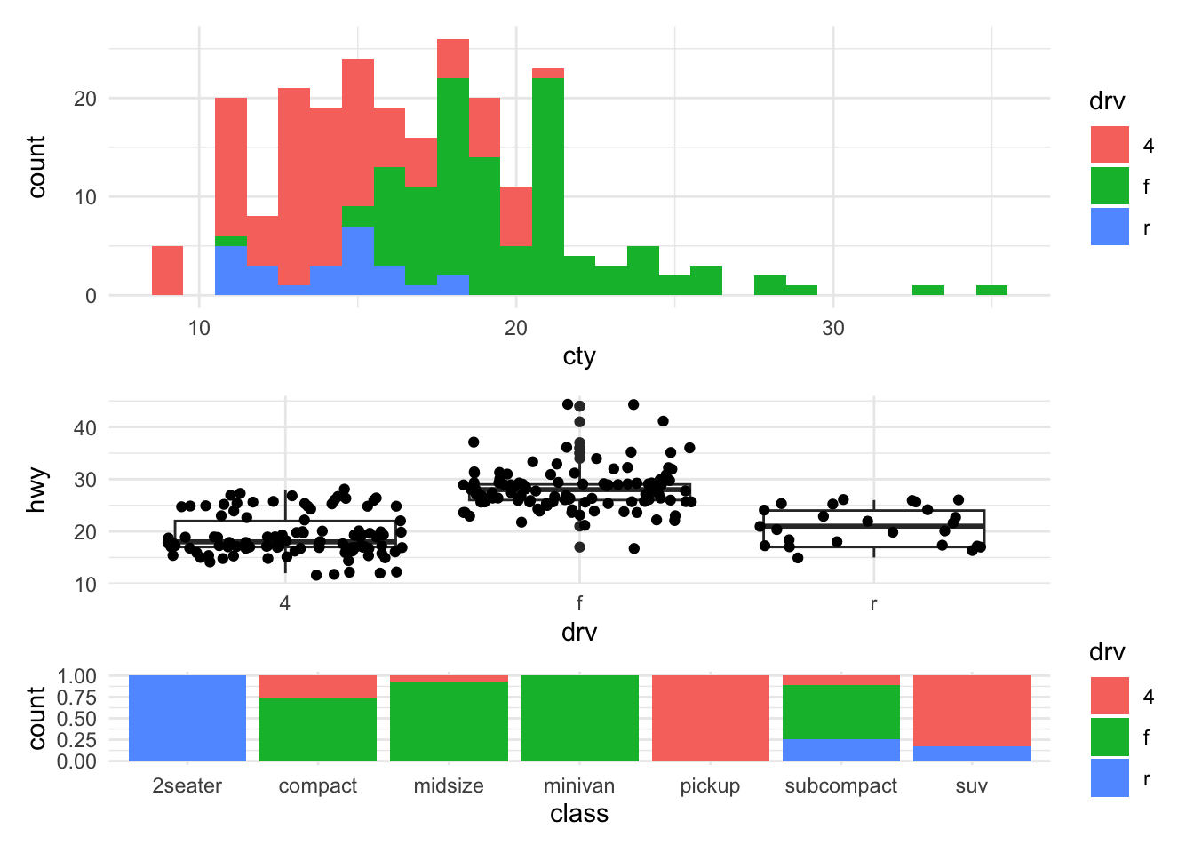
21.1.1 collapsing guides

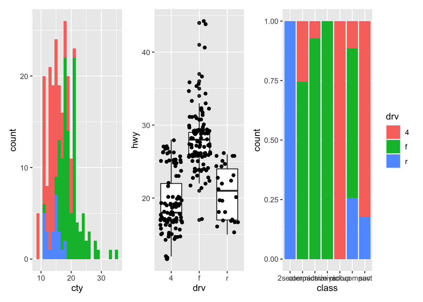
Sometimes you have multiple guides across graphs that signify the same thing. patchwork allows you to collapse the guides:

graph1 + graph2 + graph3 + plot_layout(guides = "collect")

graph1 + graph2 + guide_area() + graph3 + plot_layout(guides = "collect")

21.1.2 Showing distributions alongside scatterplots

patchwork allows nice combinations of graphs that gives the reader more insights about distributions:

hist_cty <- ggplot(mpg, aes(x = cty)) +
  geom_histogram(binwidth = 1) +
  scale_x_continuous(limits = c(8, 36), expand = c(0, 0)) +
  theme_void() +
  coord_flip()
hist_displ <- ggplot(mpg, aes(x = displ)) +
  geom_histogram(binwidth = 0.5) +
  scale_x_continuous(limits = c(1, 8), expand = c(0, 0)) +
  theme_void()
scatter <- ggplot(mpg, aes(x = displ, y = cty)) +
  geom_point() +
  scale_x_continuous(limits = c(1, 8), expand = c(0, 0)) +
  scale_y_continuous(limits = c(8, 36), expand = c(0, 0)) +
  theme_minimal()

(hist_displ | plot_spacer()) / (scatter | hist_cty)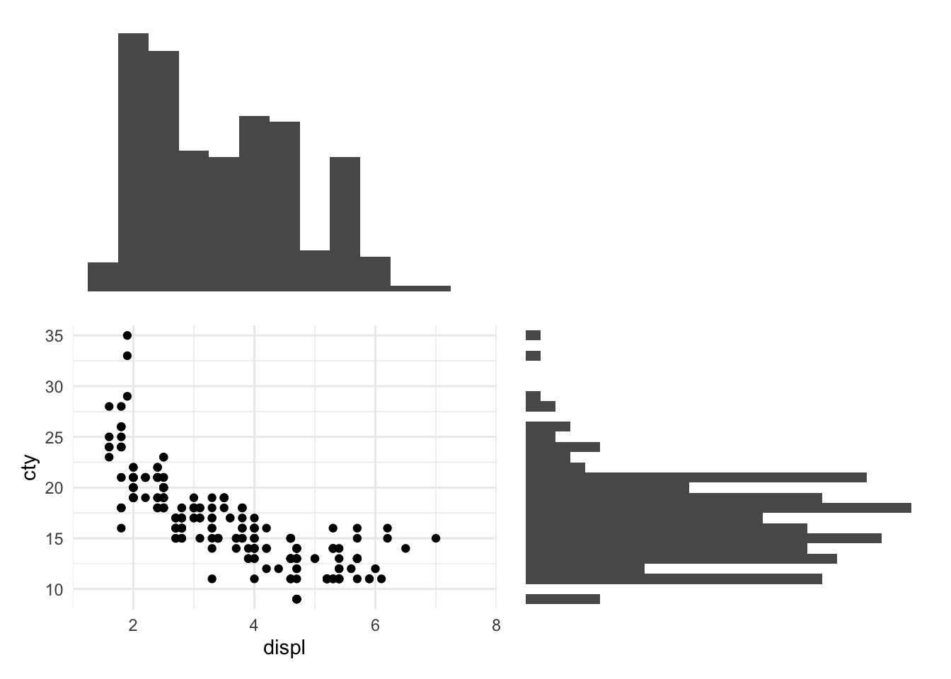

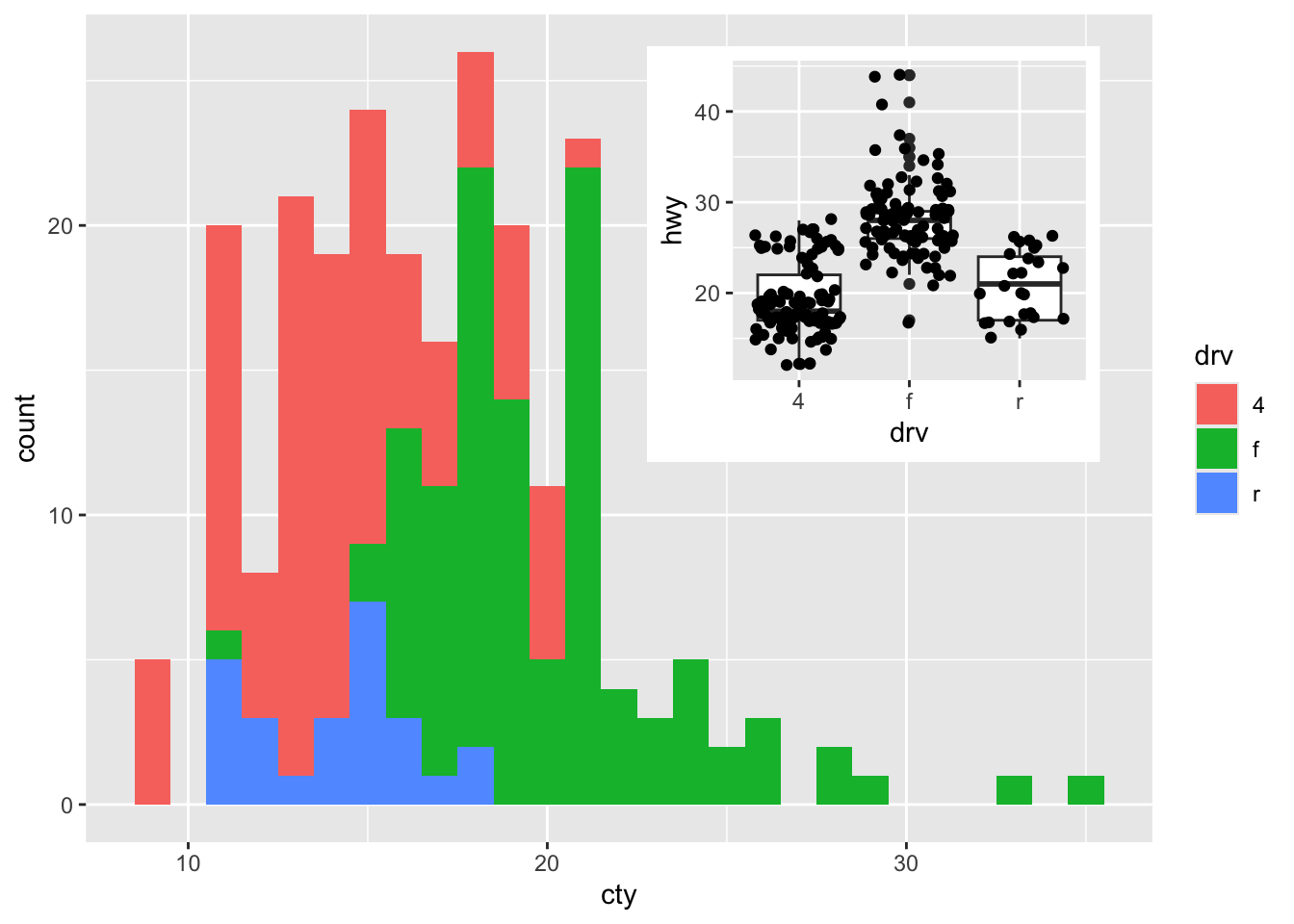
21.2 cowplot

cowplot is also a great package (see extensive documentation here. It can do some of the same things as patchwork can (albeit slighlty less intuitive), but creating insets or adding non-plots is a bit easier with this package.

install.packages("cowplot")
library(cowplot)

21.2.1 insets

insets are essentially small graphs within a graph

ggdraw(graph1) +
  draw_plot(graph2, x = .5, y = .5, width = .35, height = .45)

21.2.2 adding non-plots

We can also add non-plots, like text or images:

ggdraw() +
  draw_plot(graph2) +
  draw_label("Draft", color = "#C0A0A0", size = 100, angle = 45)

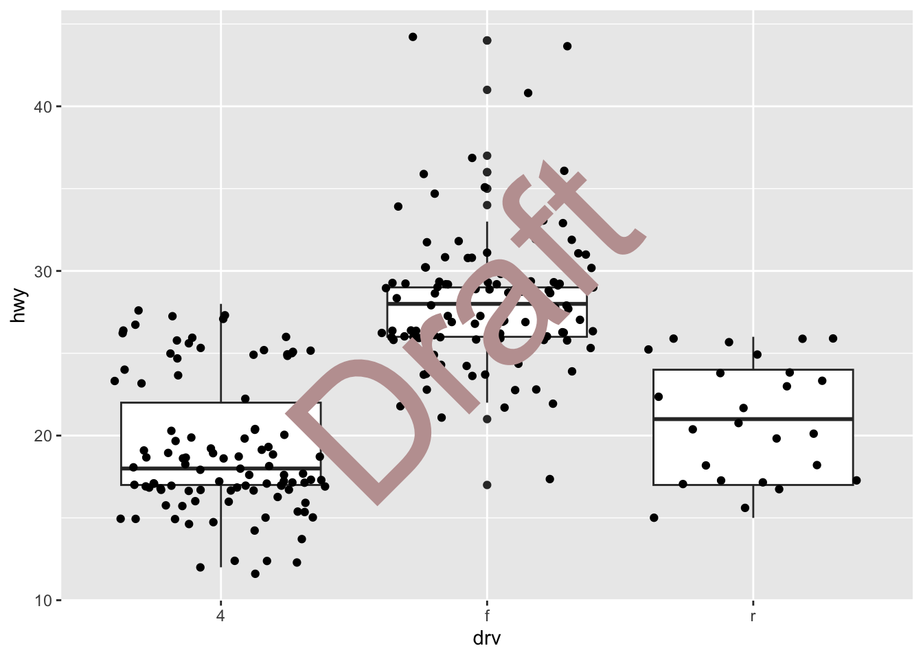
We can also add images but this requires the magick-package:

install.packags("magick")
library(magick)

img <- system.file("extdata", "cow.jpg", package = "cowplot") %>%
  image_read() %>%
  image_resize("570x380") %>%
  image_colorize(35, "white")

ggdraw() +
  draw_image(img) +
  draw_plot(graph2 + theme_minimal())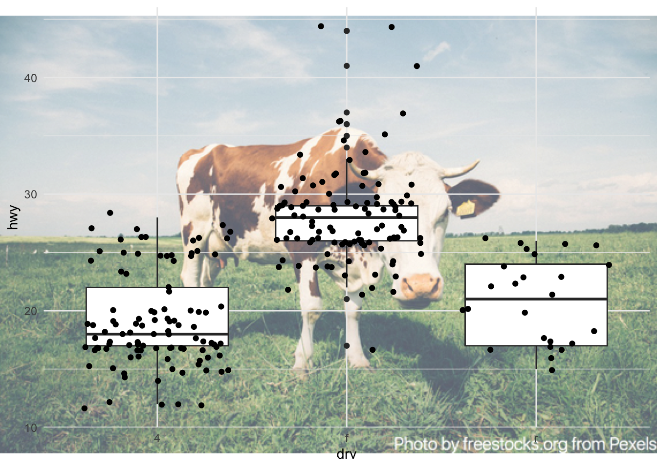

Cool stuff.