Chapter 1 R, Rstudio, and packages
Please download the most recent version of R (R Core Team 2023). RStudio will make your life much easier, so please download that too. This document was made in RStudio via R Markdown (Allaire et al. 2023), knitr (Xie 2015), and bookdown (Xie 2023).
1.1 R
R is “a freely available language and environment for statistical computing and graphics which provides a wide variety of statistical and graphical techniques”. R is thus a programming language but also an environment in which you can code and do some fancy statistical and graphical things (similar to, for instance, SPSS, Excel, or Stata).
We’ve seen several major advantages of R, but the downside of R is that it is reasonably hard to learn. R is made for statical programming and reproducible “behaviour”, not for ease of use for beginners. Particularly in the past, getting your data into R, and calculating some group means or correlations would be a significant task compared to the few clicks in SPSS. Luckily, the times, they are changing, and many developments make R much more easy to use and friendly for beginners. There is no doubt in my mind that the costs of learning R relative to other programs are well worth it compared to what you can gain from it. Even more so in this day and age where there is a major push for every part of the scientific process to be open and reproducible to others. For me personally, it was seeing the amazing graphs, and needing particular analyses that were not available in other software packages that made me move entirely to R.
1.1.1 The R-environment
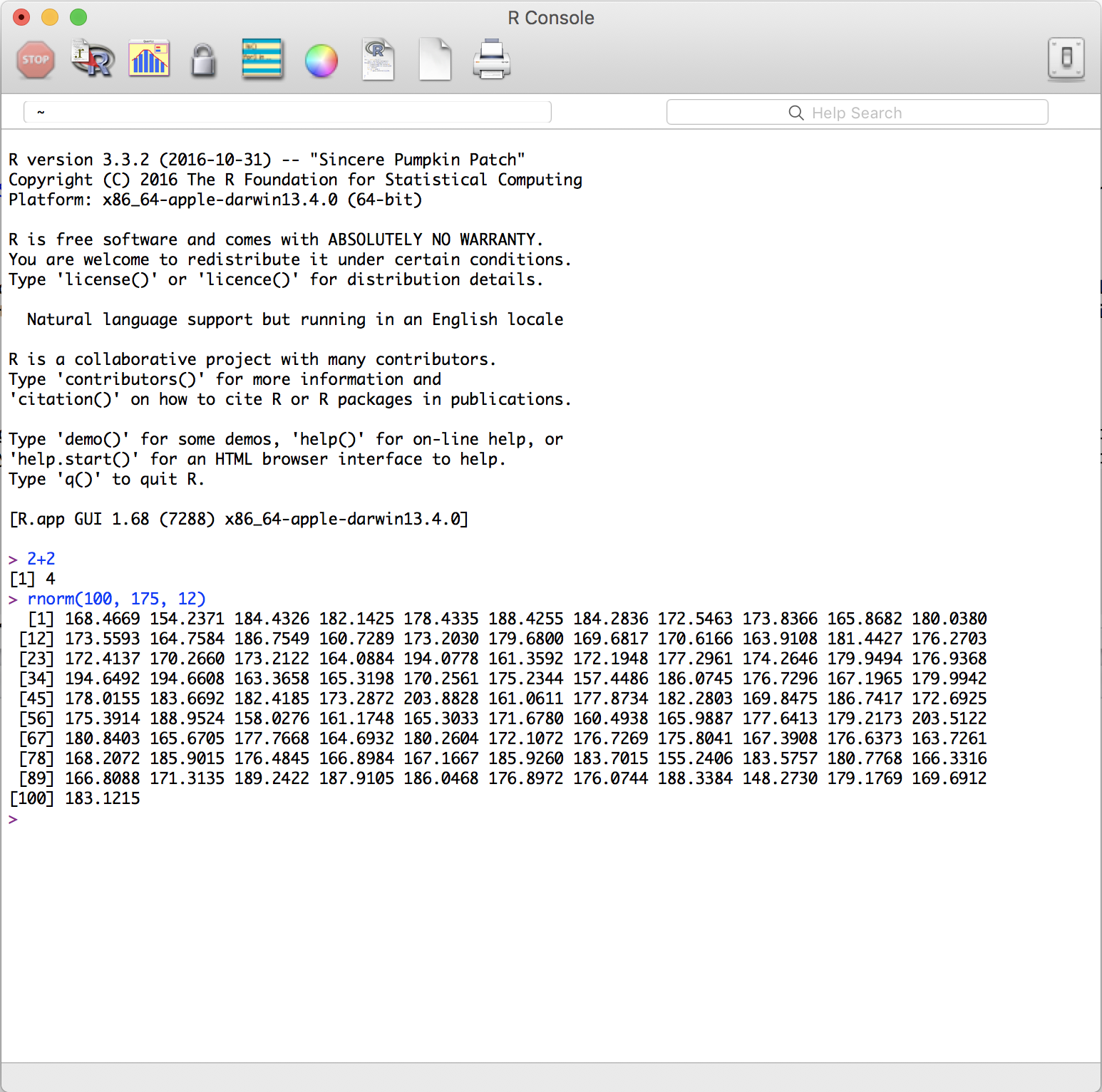
The R-environment looks very different to most other statistical software packages. This is mainly due to fact that R is “command-based” rather than “point-and-click”; this means that you have to tell R what to do with written commands, and the language that you will use for that is the R-language. In essence, you are programming when using R. The things you can do in R are near infinite. Below are two simple examples; 1) we can tell R to do add 2 and 2 (which we can do in a way that is similar to ‘natural’ language), 2) we can generate 100 numbers from a normal distribution with a mean of 175 and a standard deviation of 12 (more or less the distribution of female heights (in cm) in the Netherlands) using the “rnorm” function. This does not seem particularly useful perhaps, but the ability to generate numbers can come in handy during statistical analyses.
1.2 RStudio
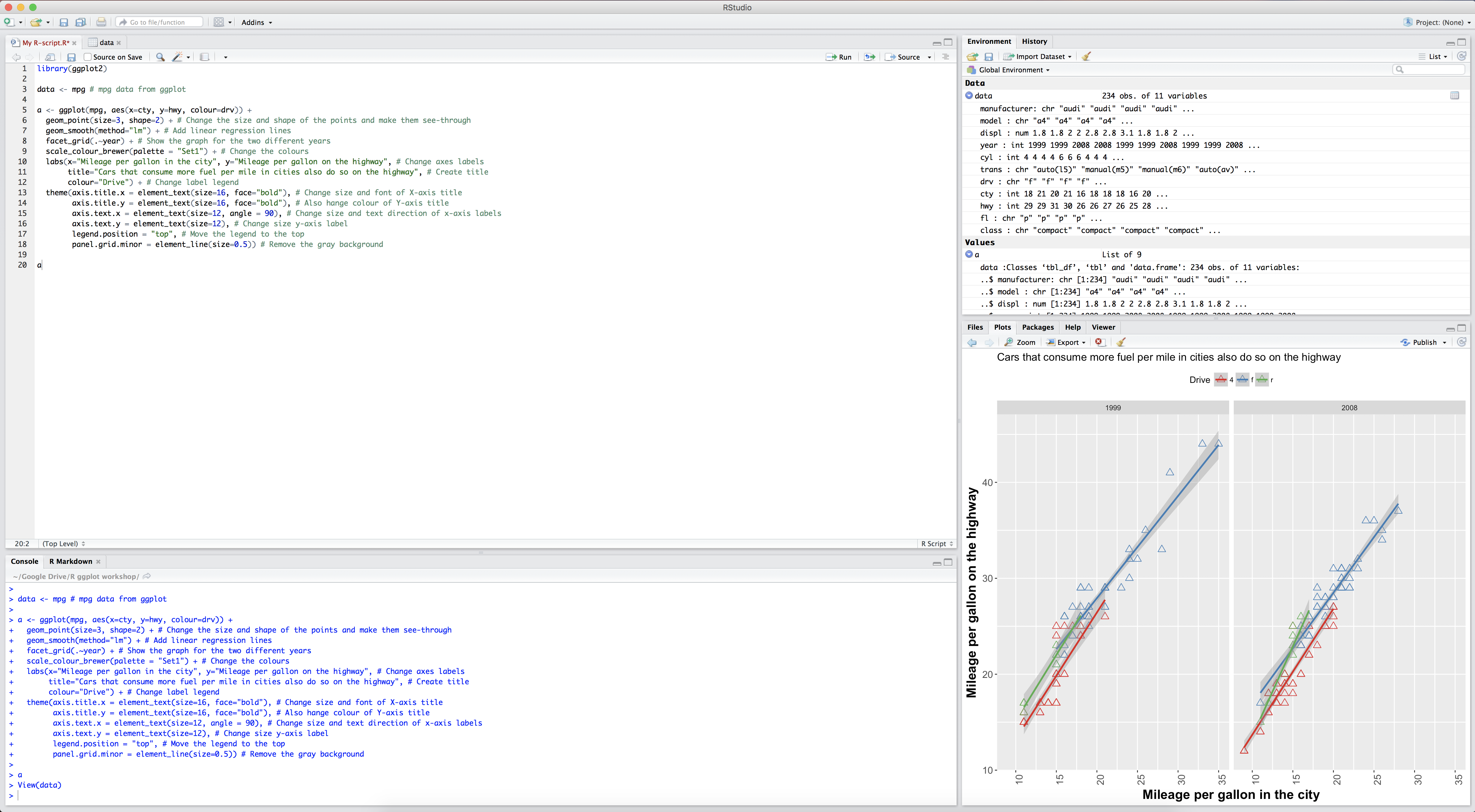
Rather than working directly in the R-environment, we’ll be working in the RStudio environment. RStudio is a free environment for working with R, that makes programming in R much, much easier. It takes away many frustrations that one might have when working in the R-environment. I myself haven’t worked in the R-environment since I discovered RStudio. An added bonus of RStudio(’s developers) is that they make many great, easy to use packages for R. In summary, download RStudio (do note that you ALSO need to have R downloaded and installed).
1.3 Installing packages
R works with “packages”. That means that for some functionality to work (like ggplot), you need to install those packages first. If you want to make use of them during your R-session, you will also need to tell R that you will be using them. You can copy all code in this document to your own R/Rstudio terminal. All the text after the hasthag “#” are comments, and will not be run by R as code.
We also need to run the packages, to let R know that we will use them in this session.
1.4 Playing around with R
Let’s go through some R-basics
You’ll see a > when you open R, or in the console from RStudio in the left bottom corner. This means that R is waiting for a command. Let’s try and do simple calculations in R. Copy the below code and run it in R.
## [1] 24R sure is good at calculating. We also see a [1] which refers to the fact that the number to the right of the [1] is the 1st element. Not very useful in this case, but we’ll see later that it can be useful.
We can perform some more complicated calculations:
## [1] 45.33882In this case, we have made use of an ‘in-built’ number (pi) and function (log). (we could obviously have done this in our heads, right?)
1.4.1 Storing objects
An important part of R is storing information in objects.
a gets assigned a 5. We see that a appears in our upper-right corner in the ‘global environment’. This means that we can use it now!
## [1] 20We could of course have stored that result as well:
And we can call on the answer.
## [1] 20We can do many other things with this object, for instance:
- is
answeridentical to the value 20?
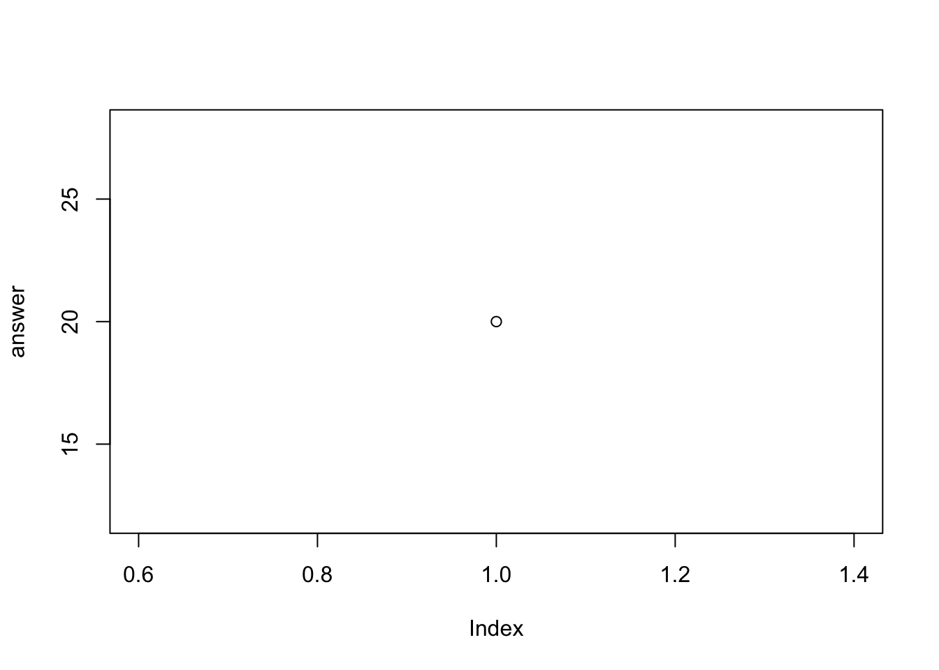
## [1] TRUE- plot the object (when it is a numeric value)
Some notes on objects:
a = 5does exactly the same thing asa <- 5; the latter option is considered better practice, because the=signs is also used to check whether an object has a particular value (e.g.,a == 5is questioning whetheraequals 5 or not.)]- There are rules to the names that you can give these objects: you can’t use spaces or special characters (e.g., ^&“’*+?); you can’t start a name with a number (i.e., you can use
object1as an object name, but not1object); capitalization matters (i.e.,myobjectis different frommyObjectwhich is different fromMyobject). - Strive for consistency in naming; I typically use lowercase and underscores (e.g.,
education_male,income_female,year_birth)
1.4.2 Functions
Above we have made use of two (built-in) function in R, namely log() and plot(). Functions take arguments and do something with these.
Functions always look something like name_function(argument1, argument2, ...). The brackets mean that we are dealing with a function, the arguments mean that the function is expecting something. Sometimes the arguments are mandatory, sometimes they are optional. Let’s look at another function in R, the round()-function, which let’s you round numbers.
Let’s call on round without any arguments:
## Error in eval(expr, envir, enclos): 0 arguments passed to 'round' which requires 1 or 2 argumentsClearly, at least one argument is rounded. Let’s round the number pi, which is stored in R as pi:
## [1] 3We can also add another argument, namely the number of decimal places we want to round off:
## [1] 3.14[this would have also worked round( pi, 2 )]
If we want information about a function, we can type the following: