Chapter 23 Shiny
This wonderful section on Shiny was co-written by Christian Luz (c.f.luz@umcg.nl)
Shiny is an R package that makes it easy to build interactive web apps straight from R. Shiny apps can be run in RStudio, embedded in RMarkdown documents, or deployed to a web server (e.g. shinyapps.io). It is a great way to interact with your data. The functionality and creativity is almost endless (check https://shiny.rstudio.com/gallery/). See also: https://www.showmeshiny.com/.
For today’s course we will build a small first shiny app to explore data from the gapminder package. Remember this code?
And this one?
ggplot(gapminder, aes(x = year, y = lifeExp)) +
  geom_line(aes(group = country)) +
  geom_line(stat = "summary", fun = "mean", colour = "blue", size = 2) +
  geom_line(data = NL, colour = "orange")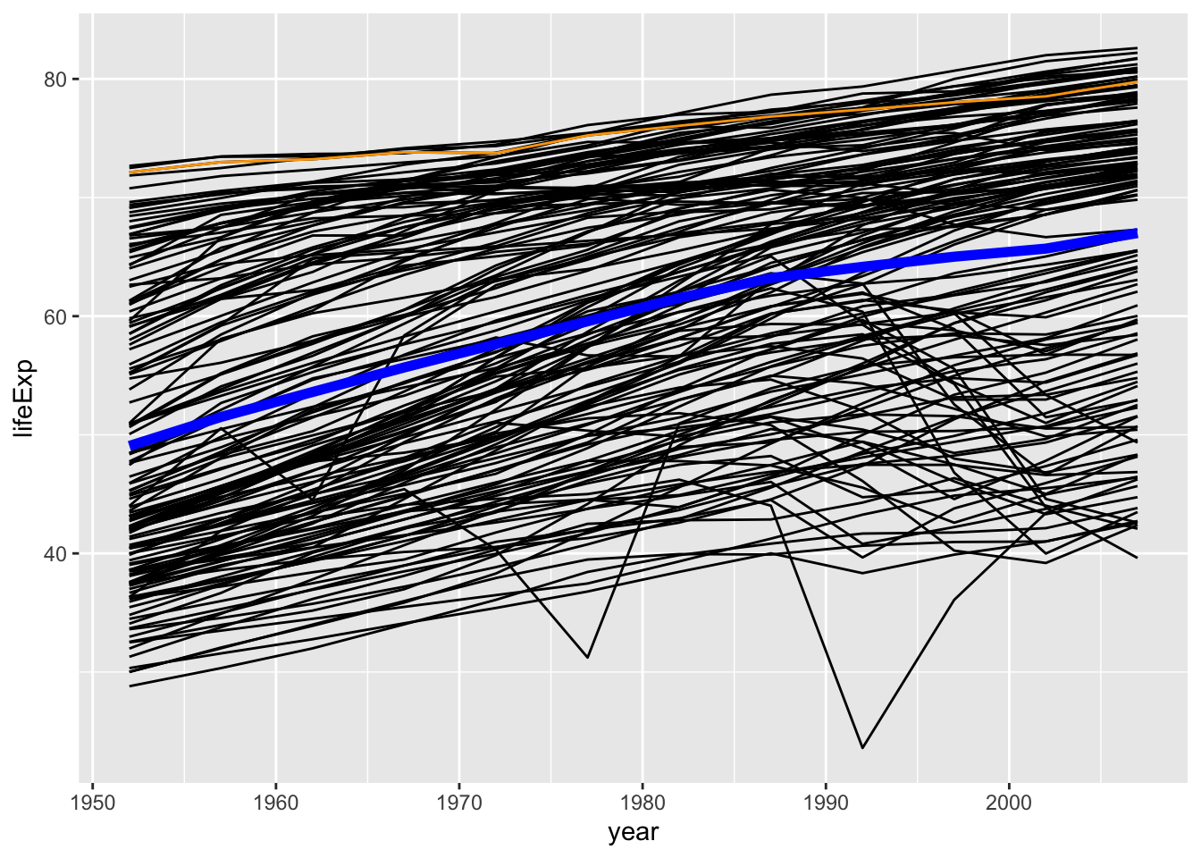
Wouldn’t it be great to have a small app to explore this data with a few simple clicks? You could also immediately communicate your findings with non-coders not as knowledgeable in R like you are now.
23.1 Creating the shiny app framework
First we need to download the shiny package.
RStudio has an easy way to initialize a shiny app. Go to File > New File > Shiny Web App… , give your app a name and select Multiple Files. Every shiny app exist of two components: the “front-end” ui.R where you define the design of your app and the “back-end” server.R where you code all your calculations, plots etc. These two components communicate with each other in a reactive way. That means they pass information from the ui (input) to the server and back (output). This fundamental difference to “normal” R scripts also requires us to write slightly different code.
When you have created the shiny template in RStudio you should have two open R scripts. Now delete all their content! :) (You could of course also just create two empty scripts and name them server.R and ui.R)
Like in every R script we need to load the packages we are going to use. Most importantly the shiny package. We also need to do this for every file (ui and server) separately.
library(shiny)
library(dplyr) # data transformation
library(ggplot2) # plotting
library(gapminder) # data source

# remember to load packages in each file: ui.R and server.R
Next we are defining the ui layout:
shinyUI(
    fluidPage(
      # here we are going to add our UI elements like checkboxes, sliders, plots, and tables
    )
)
Followed by preparing the server side (server.R):
shinyServer(function(input, output) {
  # this is were we are going to code all data transformation and output
})
Test the result by clicking the run app button on the top of one of the scripts or by running runApp("name_of_your_app") from the console.
Congrats! You have just built your first shiny app! (it’s empty though…)
23.2 Creating some content
We start with creating a typical gapminder plot on the server side of the app. We can just copy the code from above, but this time we want to send the output of the plot to the ui. We therefore need to create an output object output$plot. This object contains a call to render our plot. We use the renderPlot function from the shiny package. It takes an expression as first argument which will be our ggplot code.
# this is how your server side should look like
shinyServer(function(input, output) {

    NL <- gapminder %>% filter(country == "Netherlands")

    output$plot <- renderPlot(
        ggplot(gapminder, aes(x = year, y = lifeExp)) +
            geom_line(aes(group = country)) +
            geom_line(
              stat = "summary", fun = "mean",
              colour = "blue", size = 2
            ) +
            geom_line(data = NL, colour = "orange")
    )
})
On the ui side we need a call to display this output in our app.
Great! Try to run the app again. You should be seeing the plot from above in your app. Just a static plot - let’s add some interactivity.
23.3 Reactive input
Before we interact with the data we are going to structure the design of our app. Typically, a web app or website contains some sort of sidebar and a main panel to display some content. The shiny package comes with two functions for that: sidebarLayout and mainPanel. Within the sidebar we also add a sidebar panel (sidebarPanel). This panel will list all our input functions. We also wrap our output in the mainPanel function.
shinyUI(
    fluidPage(
        sidebarLayout(
            sidebarPanel(
              # this is were we are going to define the input
            ),
            mainPanel(
                plotOutput("plot")
            )
        )
    )
)
Empty sidebar, time to add some input widgets (https://shiny.rstudio.com/tutorial/written-tutorial/lesson3/). This is where the creativity really begins. Let’s say we want to play around with different countries in our plot. We want some form of control over the country variable in our plot. The select box could be a good choice (selectInput). Add it to the sidebar panel:
# shinyUI(
#     fluidPage(
#         sidebarLayout(
#             sidebarPanel(
              selectInput(inputId = "country", # essential! give the input a name that you will need on the server side
                        label = "Select country", # text displayed in your app
                        choices = unique(gapminder$country), # input to choose from, here all gapminder countries
                        selected = "Netherlands") # define default
#             ),
#             mainPanel(
#                 plotOutput("plot")
#             )
#         )
#     )
# )
Looks good! Now we need to go back to the server side and make use of this input selection. The value of the selected input can be used on the server side by referring to with input$variable where variable is the inputId we defined on the ui side. So, for our app that is input$country.
Now, it gets a bit more tricky. In order to interpret this information on the server side we need to tell the server that this is reactive input. That means the input is dynamic and can change. We need to wrap the filter operation in the reactive function from the shiny package and replace "Netherlands" with the new input:
This will transform NL to a reactive object. From now on the ggplot function will no longer recognize NL. Any call for the new reactive object will need to be made like this: NL() (basically looks like a function now). Let’s change the plotting code.
We also change the plot a bit to better highlight the selected country.
output$plot <- renderPlot(
ggplot(gapminder, aes(x = year, y = lifeExp)) +
geom_line(aes(group = country), colour = "lightgrey") +
geom_line(data = NL(), colour = "red", size = 1.5) +
theme_minimal()
)Perfect! That’s an interactive shiny app!
Now, we are ready to add more functionality. How about some radio buttons (radioButtons) to select different variables? Just add this to your sidebar panel (don’t forget a comma to separate the input functions).
radioButtons(
inputId = "variable",
label = "Pick parameter",
choiceNames = c("Life expectancy", "Population", "GDP per capita"), # display options
choiceValues = c("lifeExp", "pop", "gdpPercap") # actual values passed to the server
)Try to change the plotting code to use input$variable instead of lifeExp. Does it work?
No?
That’s tricky. We also need to change the aes to be able to use reactive variables. This does the trick (aes_string):
23.4 Bonus
From here you can go on and play around with shiny and make use of its enormous potential. Keep it simple or blow it up to something like this: https://ceefluz.shinyapps.io/radar/
Below some add-on code for this little gapminder app.
library(shiny)
library(gapminder)
library(DT)
shinyUI(
fluidPage(
# Application title
titlePanel("SHINY GAPMINDER"),
# Sidebar
sidebarLayout(
sidebarPanel(
selectInput(inputId = "country",
label = "Select country",
choices = unique(gapminder$country),
multiple = TRUE,
selected = "Netherlands"),
radioButtons(inputId = "variable",
label = "Pick parameter",
choiceNames = c("Life expectancy", "Population", "GDP per capita"),
choiceValues = c("lifeExp", "pop", "gdpPercap"))
),
# Output
mainPanel(
plotOutput("plot"),
checkboxInput(inputId = "continent",
label = "Show continents",
value = FALSE),
dataTableOutput("table")
)
)
)
)library(shiny)
library(tidyverse)
library(gapminder)
library(DT)
shinyServer(function(input, output) {
NL <- reactive(
  gapminder %>%
    filter(country == input$country)
)
output$plot <- renderPlot(
ggplot(gapminder, aes_string("year", input$variable,
group = "continent", fill = "continent")) +
{if(input$continent == TRUE) {
geom_smooth(method = "lm", alpha = 0.3, colour = "lightgrey")
} else {
NULL
}} +
scale_fill_manual(values = c("#D8B70A", "#02401B", "#A2A475",
"#81A88D", "#972D15")) +
geom_line(data = NL(),
aes_string("year", input$variable,
group = "country", colour = "country"),
size = 1.5) +
scale_colour_manual(values = c("red", "orange", "blue")) +
labs(fill = "Continent",
colour = "Selected country") +
theme_minimal()
)
output$table <- renderDataTable(
NL()
)
})